 "
"
Team:Groningen/modeling Spatial.html
From 2008.igem.org
| (6 intermediate revisions not shown) | |||
| Line 22: | Line 22: | ||
</li> | </li> | ||
<li class="sub"> | <li class="sub"> | ||
| - | <a href=" | + | <a href=""> Modeling </a> |
<ul Class="L2"> | <ul Class="L2"> | ||
<li class="sub"><a href="https://2008.igem.org/Team:Groningen/modeling_SingleCell.html"> Single-cell </a></li> | <li class="sub"><a href="https://2008.igem.org/Team:Groningen/modeling_SingleCell.html"> Single-cell </a></li> | ||
| Line 34: | Line 34: | ||
<li class="sub"><a href="https://2008.igem.org/Team:Groningen/results.html#results"> Results </a></li> | <li class="sub"><a href="https://2008.igem.org/Team:Groningen/results.html#results"> Results </a></li> | ||
<li class="sub"><a href="https://2008.igem.org/Team:Groningen/results.html#conclusion"> Conclusion </a></li> | <li class="sub"><a href="https://2008.igem.org/Team:Groningen/results.html#conclusion"> Conclusion </a></li> | ||
| + | <li class="sub"><a href="https://2008.igem.org/Team:Groningen/iGEM_Criteria">iGEM Criteria</a></li> | ||
</ul> | </ul> | ||
</li> | </li> | ||
| Line 48: | Line 49: | ||
</div> | </div> | ||
</div> | </div> | ||
| + | <div id="modeling_Spatial" class="location"> | ||
<div id="view"> | <div id="view"> | ||
<div id="textblock"> | <div id="textblock"> | ||
| Line 80: | Line 82: | ||
of the activators/inhibitors of the promoter. | of the activators/inhibitors of the promoter. | ||
In this way, each of the producing parts that depend on promoter activation or inhibition can be modeled | In this way, each of the producing parts that depend on promoter activation or inhibition can be modeled | ||
| - | using a single Hill Equation of the form equation 1 for promoters that are activated by | + | using a single Hill Equation of the form equation 1 for promoters that are activated by S<span class="sub">a</span> and equation 2 for |
| - | promoters that are inhibited by | + | promoters that are inhibited by S<span class="sub">i</span>. Where Vmax represents the maximal expression (without inhibition and/ |
| - | or maximal activation) of the protein and the parameter | + | or maximal activation) of the protein and the parameter K<span class="sub">m</span> represents the concentration of the inhibitor/ |
activator at which the production rate is half-maximal.</p> | activator at which the production rate is half-maximal.</p> | ||
| Line 101: | Line 103: | ||
<p> | <p> | ||
The parameters needed for our model have been taken mostly from a single paper | The parameters needed for our model have been taken mostly from a single paper | ||
| - | <span class="refcontainer">[24]<div class="reference">S. Basu, Y. Gerchman, C.H. Collins, F.H. Arnold, and R. Weiss. A synthetic multicellular system for | + | <span class="refcontainer">[24]<div class="reference">S. Basu, Y. Gerchman, C.H. Collins, F.H. Arnold, and R. Weiss. A synthetic multicellular system for programmed pattern formation. Nature, 434(7037):1130–1134</div></span> |
. and estimated from the values found there. Other sources for parameters are | . and estimated from the values found there. Other sources for parameters are | ||
| - | <span class="refcontainer">[9]<div class="reference">S. Basu, R. Mehreja, S. Thiberge, M. T. Chen, and R. Weiss. Spatiotemporal control of gene expression with pulse-generating networks. PNAS | + | <span class="refcontainer">[9]<div class="reference">S. Basu, R. Mehreja, S. Thiberge, M. T. Chen, and R. Weiss. Spatiotemporal control of gene expression with pulse-generating networks. PNAS US<span class="sub">a</span>, 101(17):6355–6360, April 2004.</div></span> |
and | and | ||
<span class="refcontainer">[25]<div class="reference">D. Braun, S. Basu, and R. Weiss. Parameter estimation for two synthetic gene networks: a case study. Acoustics, Speech, and Signal Processing, Proceedings (ICASSP ’05), 5. IEEE International Conference, March 2005</div></span> | <span class="refcontainer">[25]<div class="reference">D. Braun, S. Basu, and R. Weiss. Parameter estimation for two synthetic gene networks: a case study. Acoustics, Speech, and Signal Processing, Proceedings (ICASSP ’05), 5. IEEE International Conference, March 2005</div></span> | ||
| Line 118: | Line 120: | ||
<h3>LuxR</h3> | <h3>LuxR</h3> | ||
<p> | <p> | ||
| - | Because LuxR is constitutively expressed, we simply keep the concentration of LuxR constant at 0. | + | Because LuxR is constitutively expressed, we simply keep the concentration of LuxR constant at 0.5μM. This |
| - | + | S<span class="sub">a</span>me approach is used in | |
| - | <span class="refcontainer">[24]<div class="reference">S. Basu, Y. Gerchman, C.H. Collins, F.H. Arnold, and R. Weiss. A synthetic multicellular system for | + | <span class="refcontainer">[24]<div class="reference">S. Basu, Y. Gerchman, C.H. Collins, F.H. Arnold, and R. Weiss. A synthetic multicellular system for programmed pattern formation. Nature, 434(7037):1130–1134</div></span> |
for the wild-type LuxR. | for the wild-type LuxR. | ||
</p> | </p> | ||
| Line 127: | Line 129: | ||
HSL and LuxR have to form a complex first before they can form the HSL.LuxR complex, this is modeled in de | HSL and LuxR have to form a complex first before they can form the HSL.LuxR complex, this is modeled in de | ||
ODE by quadratizing both terms | ODE by quadratizing both terms | ||
| - | <span class="refcontainer">[24]<div class="reference">S. Basu, Y. Gerchman, C.H. Collins, F.H. Arnold, and R. Weiss. A synthetic multicellular system for | + | <span class="refcontainer">[24]<div class="reference">S. Basu, Y. Gerchman, C.H. Collins, F.H. Arnold, and R. Weiss. A synthetic multicellular system for programmed pattern formation. Nature, 434(7037):1130–1134</div></span> . |
</p> | </p> | ||
<div class="formula" id="ODE3"><img src="https://static.igem.org/mediawiki/igem.org/d/d3/Groningen2008_ODE3.png" /></div> | <div class="formula" id="ODE3"><img src="https://static.igem.org/mediawiki/igem.org/d/d3/Groningen2008_ODE3.png" /></div> | ||
| Line 144: | Line 146: | ||
can be found on the website and contains all the listed ODE functions. | can be found on the website and contains all the listed ODE functions. | ||
To study the response of our model we included sender populations, referred to below as sender cells, in our | To study the response of our model we included sender populations, referred to below as sender cells, in our | ||
| - | spatial grid. These populations constantly produce | + | spatial grid. These populations constantly produce 1μM of HSL and are depicted in the images as red cells. |
Because we are interested in the steady states, the images shown are snapshots taken after running the | Because we are interested in the steady states, the images shown are snapshots taken after running the | ||
model for approximately 1000 time-steps (minutes). | model for approximately 1000 time-steps (minutes). | ||
| Line 167: | Line 169: | ||
<h3>Decreasing lux Promoter Sensitivity</h3> | <h3>Decreasing lux Promoter Sensitivity</h3> | ||
<p>After setting the concentration of HSL.LuxR that is needed for half-maximal expression of CI twice as high | <p>After setting the concentration of HSL.LuxR that is needed for half-maximal expression of CI twice as high | ||
| - | (to 0. | + | (to 0.16μM), we get the result shown in Figure 6.9. There we can see that more HSL is required to produce |
enough CI to inhibit GFP output, slightly increasing the width of the band.</p> | enough CI to inhibit GFP output, slightly increasing the width of the band.</p> | ||
<table class="image-right"> | <table class="image-right"> | ||
<caption align="bottom"> | <caption align="bottom"> | ||
| - | Figure 6.9. GFP response with a single sender cell, with | + | Figure 6.9. GFP response with a single sender cell, with K<span class="sub">l(a)</span>increased |
| - | to 0. | + | to 0.16μM. |
</caption> | </caption> | ||
<tr><td><img src="https://static.igem.org/mediawiki/igem.org/1/19/Groningen2008_Figure69.png" /></td></tr> | <tr><td><img src="https://static.igem.org/mediawiki/igem.org/1/19/Groningen2008_Figure69.png" /></td></tr> | ||
| Line 194: | Line 196: | ||
not show a GFP response, and when only a single neighboring cell is ON, a cell does show a GFP response. | not show a GFP response, and when only a single neighboring cell is ON, a cell does show a GFP response. | ||
After playing around with the parameters we found that one way of achieving this behavior is by drastically | After playing around with the parameters we found that one way of achieving this behavior is by drastically | ||
| - | decreasing HSL diffusion to 0.00001 | + | decreasing HSL diffusion to 0.00001 mm<span class="super">2</span> min<span class="super">-1</span> and increasing HSL decay to 0.03 min<span class="super">-1</span>, the resulting snapshot |
| - | of the grid is shown in Figure 6.11 | + | of the grid is shown in Figure 6.11. </p> |
| - | + | ||
| - | + | ||
| Line 203: | Line 203: | ||
<caption align="bottom"> | <caption align="bottom"> | ||
Figure 6.11. GFP response with two sender cells. HSL diffusion set to | Figure 6.11. GFP response with two sender cells. HSL diffusion set to | ||
| - | 0. | + | 0.00001mm<span class="super">2</span> min<span class="super">-1</span> and HSL decay set to 0.03 min<span class="super">-1</span>. |
</caption> | </caption> | ||
<tr><td><img src="https://static.igem.org/mediawiki/igem.org/c/c4/Groningen2008_Figure611.png" /></td></tr> | <tr><td><img src="https://static.igem.org/mediawiki/igem.org/c/c4/Groningen2008_Figure611.png" /></td></tr> | ||
</table> | </table> | ||
| + | <p>A nice thing to note is that such parameter-tweaks can also be done | ||
| + | in ’real biology’ like by modifying the pH of the solution to increase HSL decay or increasing the density of the | ||
| + | medium or distance between cells to reduce HSL diffusion speed.</p> | ||
| Line 214: | Line 217: | ||
</div> | </div> | ||
</div> | </div> | ||
| + | </div> | ||
<html> | <html> | ||
Latest revision as of 03:08, 30 October 2008

Modeling: Spatial Approach
Introduction
In this chapter we will present the model we used to do spatial simulations of our interval switch network. This network is intended as part of a cellular automaton that serve as a detector that can differentiate between having ’too few’ and ’too many’ neighbors, in this chapter we will try to demonstrate this concept for the case where no neighbors is ’too few’ and two neighbors is ’too many’.
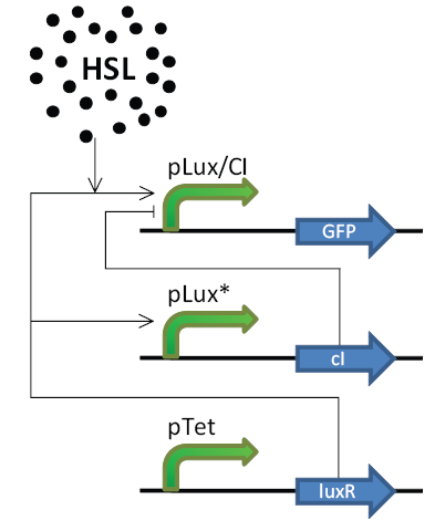
Network Overview
The network we simulate is shown in Figure 6.7. It consists of one hybrid promoter, inhibited by CI and activated by HSL.LuxR, which facilitates GFP expression. The second promoter is a modified lux promoter which is activated by HSL.LuxR and facilitates CI expression. Because the lux promoter is modified in such a way that the binding site is less easily bound to, we expect that more HSL.LuxR is needed to express enough CI to block the hybrid promoter. This means that when HSL. LuxR is too low, the hybrid promoter (and GFP expression) will not be turned on, and when HSL.LuxR exceeds a certain treshold, the lux promoter will be activated and its CI expression will block the hybrid promoter, stopping GFP expression. The result is a network that will only show a GFP response if the HSL.LuxR concentration is inbetween two limits.
 |
Spatial Model
In this section we will give a specification of our model on a ’high level’, meaning that each sensing and protein
producing part is modelled as a single Ordinary Differential Equation (ODE) using Hill equations
[23]
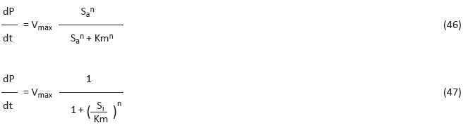
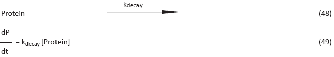
Of course we also have to model ’standard’ linear reactions such as decay (reaction 48). We do this using Mass Action (MA) kinetics (resulting in equation 49). Note that species depicted in brackets [], represent the concentration.
In the following subsections we will present the model we used to simulate the behavior of our gene network. The Matlab source code itself can be downloaded from 'Modeling Files'
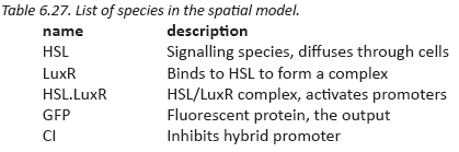
Species
This section lists the different species that are present in the model.
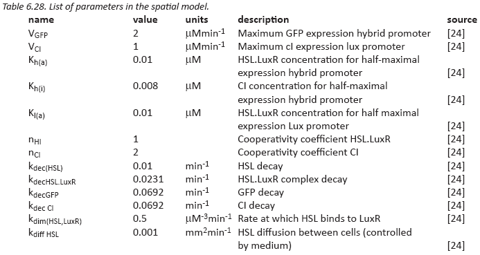
Parameters
The parameters needed for our model have been taken mostly from a single paper
[24]
Ordinary Differential Equations
In this section we list the Differential Equations that make up our model. Species depicted in brackets [], depict the concentration of a substance. Each differential equation represents the derivative of the concentration of a substance, in other words the production of a species at a single time-step.
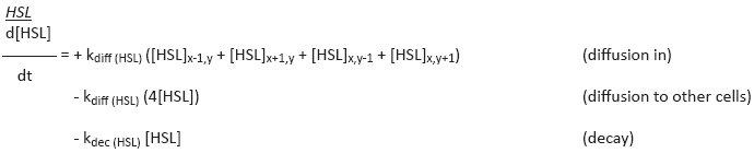
These ODEs take into account the diffusion of HSL to and from other cells (the current cell is (x,y)). For this model we consider a 2-dimensional grid and it is assumed that each cell has four neighboring cells.
LuxR
Because LuxR is constitutively expressed, we simply keep the concentration of LuxR constant at 0.5μM. This
Same approach is used in
[24]
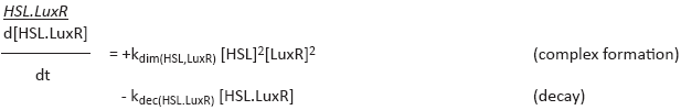
HSL and LuxR have to form a complex first before they can form the HSL.LuxR complex, this is modeled in de
ODE by quadratizing both terms
[24]
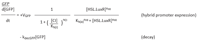
GFP response depends on HSL.LuxR and CI concentrations, where the first acts as an activator and the second serves as an inhibitor.
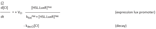
The amount of CI expressed depends on the modified lux promoter, meaning that expression is activated by the amount of HSL.LuxR. Because this promoter is weaker then the promoter that activates GFP expression, i.e. it needs more HSL.LuxR, we can create a band of HSL.LuxR concentrations where GFP is expressed but CI is not yet (sufficiently) expressed.
Simulations
To solve this collection of ODEs we used MATLAB’s
[11]
Single Sender Cell Simulations
Standard Parameters
When we simply run our model with the parameters described in the paper and include a single sender cell, we get the result as shown in Figure 6.8. We can see that, as expected, a band of GFP forms around the sender cells, indicating that the cells that are near a sender get too much HSL and the cells that are far away from the sender does not get enough HSL for proper activation.
 |
Decreasing lux Promoter Sensitivity
After setting the concentration of HSL.LuxR that is needed for half-maximal expression of CI twice as high (to 0.16μM), we get the result shown in Figure 6.9. There we can see that more HSL is required to produce enough CI to inhibit GFP output, slightly increasing the width of the band.
 |
Multiple Sender Cell Simulations
Standard Parameters
When we run the model with the normal parameters and two sender cells, we get the result as shown in Figure 6.10. This indicates that cells that receive HSL from both senders now approach the high threshold and show a lesser GFP response.
 |
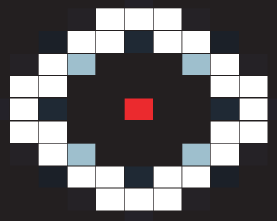
Tweaked Parameters
We now try to adjust the parameters so that we get a response that is suitable for use in a cellular automaton. In this case we try to tweak the model so that when two neighboring cells are ON, a cell does not show a GFP response, and when only a single neighboring cell is ON, a cell does show a GFP response. After playing around with the parameters we found that one way of achieving this behavior is by drastically decreasing HSL diffusion to 0.00001 mm2 min-1 and increasing HSL decay to 0.03 min-1, the resulting snapshot of the grid is shown in Figure 6.11.
 |
A nice thing to note is that such parameter-tweaks can also be done in ’real biology’ like by modifying the pH of the solution to increase HSL decay or increasing the density of the medium or distance between cells to reduce HSL diffusion speed.