Team:Montreal/Modeling
From 2008.igem.org
| Home | The Team | The Project | Parts | Modeling | Notebook | Links | Sponsors |
|---|
Modeling
Background
Using coupled differential equations, we are modeling the repressilator, which is a network of three genes, whose product proteins are repressing each other's growth. This cycle is taking place in each of a colony of cells, who communicate amongst themselves by exchanging an autoinducer molecule. The model attempts to take into account a sparse, heterogeneous distribution of cells with depletion of the autoinducer molecule and leakage.
For this purpose, the model is currently being coded up in Mathematica. The simulations, based on that continuous model, are generated using xCellerator and NDelayDSolve for different cell configurations (fig. 1); the results obtained are graphs of the concentration of molecules in the system versus time (fig. 2). That is, our interest lies in the phase difference between clusters of cells. As of now, a low number of cells is being used for testing, but a higher one will be reached later.
Journal
The Mathematica notebook used to model the repressillator incorporates xCellerator to create the differential equations representing the chemical reactions at play. The system was then solved using NDSolve, a standard numerical solver in Mathematica -- which is, however, unable to deal with delay equations. Hence, the equations were not evaluated at retarded times at first.
The first solution found was to add null cells in the network. The nulls cells, or pseudo cells, are just grid point where no internal cell reaction occurs, but only diffusion to the next grid point. However, the results depended to heavily on the number of such null cells and, as we did not have a mean of estimating what would be realistic, did not seem reliable enough.
We are now replacing NDSolve with NDelayDSolve to solve the system and we are therefore able to evaluated our equations at retarded times. We are not using null cells anymore. The value of the delays corresponds to the time the molecules of AI diffuse the intercellular distance: the reasoning being that each cells effectively "sees" the concentration of another cell at an earlier time -- the time the molecules take to diffuse between them.
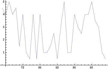
For a given distance between the two clusters of cells (fig. 1), we plot the concentration of AI in each cells versus time. From there, we extract two informations: synchronization time and phase difference (fig. 3-6). The general trend in fig. 3 seems to be that the longer the distance, the longer it takes to synchronize, but we also noticed that after a certain distance, the two clusters are no longer in synchrony. Unless they just take much longer to synchronize than the windows of the graph -- in which case we would need to run the simulation for a longer time to observe synchronization. As for the graph of the phase difference (fig. 4-6) made to different scales, we have yet to figure out what could be the pattern.
 "
"


