 "
"
Team:iHKU/modeling
From 2008.igem.org
|
||||||||||||||||||||||||||||||||
ModelingCONTENTS:
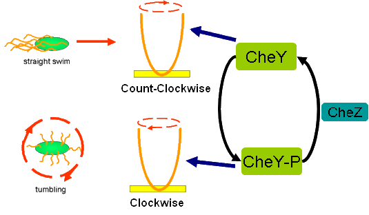
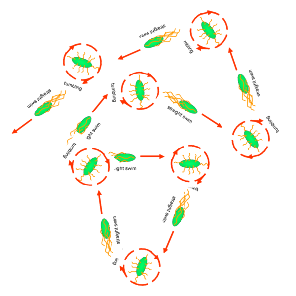
Cell Movement in Microscopic and Macroscopic AspectBasically, we considered the movement of a cell as a process of random walk, since an individual E.coli cell was always in the states between moving and tumbling (Fig.1).Similar to Brownian particles, the random walk of E.coli followed the Einstein-Smoluchowski theory [1].
Fig . 1 Genetic circuit related to cell movementin(left) and cell random walk(right)
Firstly, for the one dimension of random walk, let x (t) denote the position of an E.coli cell at time t, given that its position coincided with the point x=0 at time t=0. And we assumed an E.coli cell moves an average distance l—in either the positive or negative direction of the x-axis—each step (during a time (τ) between two tumbling states). The probability that the cell was found at the point x at time t was now equal to the probability that, in a series of n (=t/τ) successive moving steps, the cell made m more steps in the positive direction of the axis than in the negative direction. The desired probability was given by the binomial expression [1, 2]  (1.1) (1.1)
To simplify equation (1.1), for m<<n, we obtain  (1.2) (1.2)
Taking x to be a continuous variable, we can obtain  (1.3) (1.3)
where
v= l/τ was the average speed of the cell movement, and f=1/τ was the tumbling frequency of E.coli. In two dimensions, the square of the distance from the origin to the point (x, y) was r2=x2+y2; therefore
For a macroscopic view, D was defined as the diffusion coefficient. For a simple diffusion process, it is easy to write an diffusion equation to describe the density ρ distribution.  ...................................................................................................(1.4) ...................................................................................................(1.4)
Normally, as the swimming speed of E.coli is about 20um/s and the tumbling frequency is about 1 Hz, the diffusion coefficient is about 200um2/s [3].
Front propagation for cell growth
|
 ,
,
|