Team:Imperial College/Genetic Circuit
From 2008.igem.org
m |
m |
||
| Line 9: | Line 9: | ||
A simple [[Imperial_College/Courses/Spring2008/Synthetic_Biology/Computer_Modelling_Practicals/Practical_2 | synthesis-degradation model]] is assumed for the modelling of the expression of a protein under the control of a constitutive promoter, with the same model assumed for all four [[IGEM:IMPERIAL/2008/Prototype/Wetlab/test_constructs | promoter-RBS constructs]]. The synthesis-degradation model assumes a steady state level of mRNA. | A simple [[Imperial_College/Courses/Spring2008/Synthetic_Biology/Computer_Modelling_Practicals/Practical_2 | synthesis-degradation model]] is assumed for the modelling of the expression of a protein under the control of a constitutive promoter, with the same model assumed for all four [[IGEM:IMPERIAL/2008/Prototype/Wetlab/test_constructs | promoter-RBS constructs]]. The synthesis-degradation model assumes a steady state level of mRNA. | ||
| - | <math>\frac{d[protein]}{dt} | + | <math>\frac{d[protein]}{dt} {{Equals}} k_{1} - d_{1}[protein]</math> |
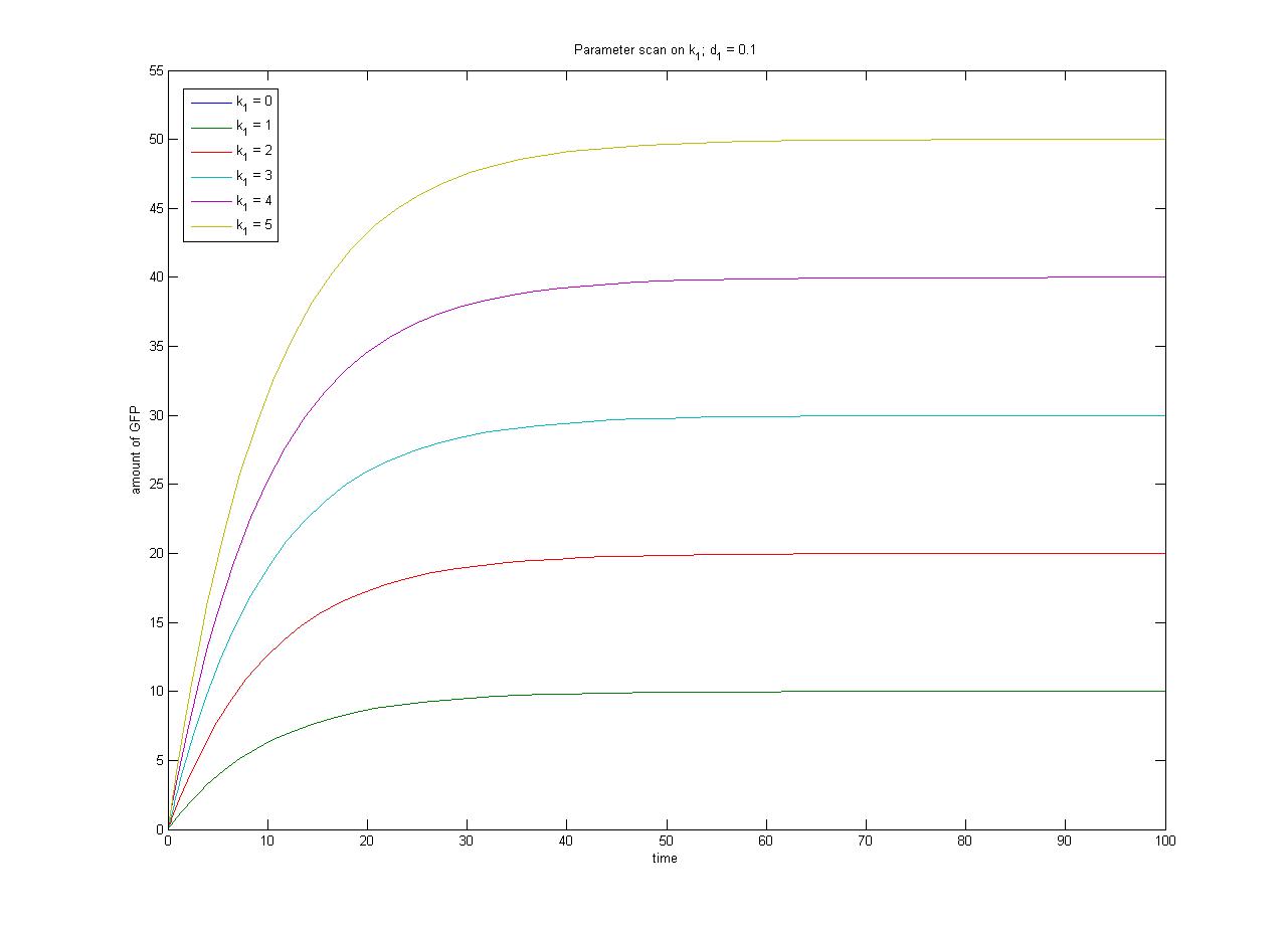
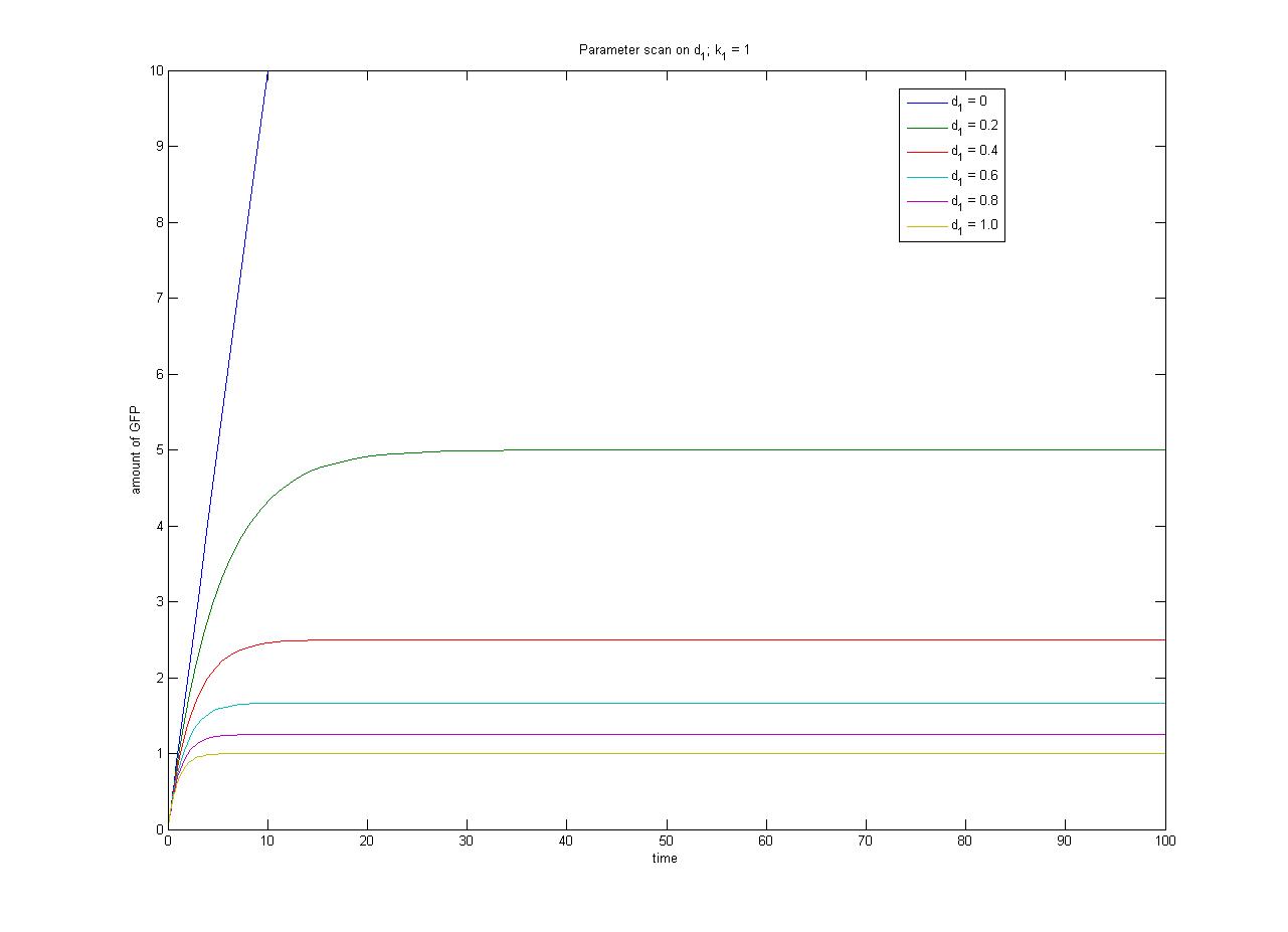
In this case, <math>[protein]</math> represents the concentration of GFP, <math>k_{1}</math> represents the rate of sythesis and <math>d_{1}</math> represents the degradation rate. | In this case, <math>[protein]</math> represents the concentration of GFP, <math>k_{1}</math> represents the rate of sythesis and <math>d_{1}</math> represents the degradation rate. | ||
| Line 19: | Line 19: | ||
We can also solve this ODE analytically. Consider the steady-state behaviour of <math>[protein]</math>. | We can also solve this ODE analytically. Consider the steady-state behaviour of <math>[protein]</math>. | ||
| - | <math>\frac{d[protein]}{dt} | + | <math>\frac{d[protein]}{dt}{{Equals}}0 \Rightarrow [protein]_{steady-state}{{Equals}}\frac{k_1}{d_1}</math> |
This relationship can be seen in the parameter scan graphs on the right. | This relationship can be seen in the parameter scan graphs on the right. | ||
| Line 26: | Line 26: | ||
<br> | <br> | ||
Note from the parameter scan graphs:<br> | Note from the parameter scan graphs:<br> | ||
| - | *In the case where <math>k_1 | + | *In the case where <math>k_1 {{Equals}} 0</math>, no GFP is sythesised. |
| - | *In the case where <math>d_1 | + | *In the case where <math>d_1 {{Equals}} 0</math>, the concentration of protein does not reach a steady state. |
|[[Image:Phase 1.PNG|thumb|300px|Constitutive expression of antibiotic resistance (AB) and GFP. GFP brick is part E0040, GFPmut3b. Terminator is part B0015, the double-stop.]] | |[[Image:Phase 1.PNG|thumb|300px|Constitutive expression of antibiotic resistance (AB) and GFP. GFP brick is part E0040, GFPmut3b. Terminator is part B0015, the double-stop.]] | ||
| - | <gallery caption | + | <gallery caption{{Equals}}"Parameter Scan" align{{Equals}}"right"> |
Image:ParamterScanGFPk1.jpg|Parameter scan on <math>k_1</math> | Image:ParamterScanGFPk1.jpg|Parameter scan on <math>k_1</math> | ||
| - | Image:ParamterScanGFPd1.jpg|Parameter scan on <math>d_1</math> | + | Image:ParamterScanGFPd1.jpg|Parameter scan on <math>d_1</math></gallery> |
| - | </gallery>}} | + | }} |
| - | {{Imperial/Box1|Modelling Inducible Gene Expression | + | {{Imperial/Box1|Modelling Inducible Gene Expression |
| - | [[Image:Phase 2-linduced.PNG|thumb|300px]] | + | |[[Image:Phase 2-linduced.PNG|thumb|300px]] |
The repressor is constitutively expressed. Hence we can assume the constitutive expression model from the previous characterisation step. | The repressor is constitutively expressed. Hence we can assume the constitutive expression model from the previous characterisation step. | ||
| - | <math>\frac{d[R]}{dt} | + | <math>\frac{d[R]}{dt} {{Equals}} k_{1} - d_{1}[R]</math> |
When the inducer is added it binds reversibly to the repressor. | When the inducer is added it binds reversibly to the repressor. | ||
| Line 48: | Line 48: | ||
Repressor only binds to the promoter when it is in its unbound form, hence transcription will be a function of free repressor concentration. | Repressor only binds to the promoter when it is in its unbound form, hence transcription will be a function of free repressor concentration. | ||
| - | <math> Transcription | + | <math> Transcription {{Equals}} \frac{\beta.{[R]}^n}{{K_m}^n+[R]^n}</math><br> |
And overall protein expression can be described as | And overall protein expression can be described as | ||
| - | <math>\frac{d[protein]}{dt} | + | <math>\frac{d[protein]}{dt} {{Equals}} Transcription - d_2[protein]</math> |
The [[media:ConcentrationsODE.m|ODEs]] and [[media:SimulationconcentrationsODE.m|simulation]] may be found in the Appendices section of the Dry Lab hub. | The [[media:ConcentrationsODE.m|ODEs]] and [[media:SimulationconcentrationsODE.m|simulation]] may be found in the Appendices section of the Dry Lab hub. | ||
<biblio> | <biblio> | ||
| - | #1 pmid | + | #1 pmid{{Equals}}18612302 |
</biblio> | </biblio> | ||
}} | }} | ||
{{Imperial/EndPage|Project|Motility}} | {{Imperial/EndPage|Project|Motility}} | ||
Revision as of 00:39, 10 October 2008
{{Imperial/Box1|Modelling Inducible Gene Expression |The repressor is constitutively expressed. Hence we can assume the constitutive expression model from the previous characterisation step. <math>\frac{d[R]}{dt} = k_{1} - d_{1}[R]</math> When the inducer is added it binds reversibly to the repressor. <math> R + I \Leftrightarrow RI </math> Repressor only binds to the promoter when it is in its unbound form, hence transcription will be a function of free repressor concentration. <math> Transcription = \frac{\beta.{[R]}^n}{{K_m}^n+[R]^n}</math> And overall protein expression can be described as <math>\frac{d[protein]}{dt} = Transcription - d_2[protein]</math> The ODEs and simulation may be found in the Appendices section of the Dry Lab hub. <biblio>
</biblio> }} |
|||||||||||||
 "
"


