|
|
| Line 1: |
Line 1: |
| | {{Imperial/StartPage2}} | | {{Imperial/StartPage2}} |
| - | <br>
| + | |
| - | <br>
| + | |
| | {{Imperial/Box2|Growth Curve| | | {{Imperial/Box2|Growth Curve| |
| | Part of our dry lab team concentrated on modelling the growth curve of ''B. subtilis''. This is important to characterise the chassis; particularly, the growth of ''subtilis'' is a vital parameter for planning experiments for future projects. Characterisation increases the predictability of the growth of B. subtilis by determining, for example, its growth rate and the duration of its distinctive growth phases. In order to model the growth of ''B. subtilis'', the process was broken down into three main steps, where a separate submodel is produced in MATLAB for each step. Each submodel is an ODE model, which can be simulated using MATLAB. The variables in each submodel can be adjusted according to the boundary conditions (from experimental results). | | Part of our dry lab team concentrated on modelling the growth curve of ''B. subtilis''. This is important to characterise the chassis; particularly, the growth of ''subtilis'' is a vital parameter for planning experiments for future projects. Characterisation increases the predictability of the growth of B. subtilis by determining, for example, its growth rate and the duration of its distinctive growth phases. In order to model the growth of ''B. subtilis'', the process was broken down into three main steps, where a separate submodel is produced in MATLAB for each step. Each submodel is an ODE model, which can be simulated using MATLAB. The variables in each submodel can be adjusted according to the boundary conditions (from experimental results). |
| | | | |
| - | In the final step, a combination of Submodels 1 and 2 are superposed with Submodel 3, resulting in a more complex model which enhances the accuracy of illustrating bacterial growth. For more details about the submodels, please click on the following links: | + | In the final step, a combination of Submodels 1 and 2 are superimposed with Submodel 3, resulting in a more complex model which enhances the accuracy of illustrating bacterial growth. For more details about the submodels, please see the [[Team:Imperial_College/Appendices | Dry Lab Appendices page]]. |
| - | | + | |
| - | | + | |
| - | '''[[Tutorial for Growth Curve]]''' (More details about each submodel)
| + | |
| - | | + | |
| - | '''[[Media:Modelling_Growth_Curve.pdf]]''' (The tutorial questions)
| + | |
| | | | |
| | The graph on the right shows the log graph used to determine the growth rate. | | The graph on the right shows the log graph used to determine the growth rate. |
| Line 17: |
Line 11: |
| | {{Imperial/Box1|Key Phases of Bacterial Growth| | | {{Imperial/Box1|Key Phases of Bacterial Growth| |
| | ===Lag Phase=== | | ===Lag Phase=== |
| - | During the lag phase, the rate of growth is slow due to two main reasons, ''B. subtilis'' is absorbing nutrients in the medium and the replication machinery is being switched on. The higher the concentration of nutrients in the medium, the faster the rate of bateria growth. | + | During the lag phase, the rate of growth is slow due to two main reasons, ''B. subtilis'' is absorbing nutrients in the medium and the replication machinery is being switched on. The higher the concentration of nutrients in the medium, the faster the rate of bacteria growth. |
| | | | |
| | As a result, the volume of the bacteria increases, followed by an increase in the number of bacteria. | | As a result, the volume of the bacteria increases, followed by an increase in the number of bacteria. |
|
| Growth Curve
|
|
Part of our dry lab team concentrated on modelling the growth curve of B. subtilis. This is important to characterise the chassis; particularly, the growth of subtilis is a vital parameter for planning experiments for future projects. Characterisation increases the predictability of the growth of B. subtilis by determining, for example, its growth rate and the duration of its distinctive growth phases. In order to model the growth of B. subtilis, the process was broken down into three main steps, where a separate submodel is produced in MATLAB for each step. Each submodel is an ODE model, which can be simulated using MATLAB. The variables in each submodel can be adjusted according to the boundary conditions (from experimental results).
In the final step, a combination of Submodels 1 and 2 are superimposed with Submodel 3, resulting in a more complex model which enhances the accuracy of illustrating bacterial growth. For more details about the submodels, please see the Dry Lab Appendices page.
The graph on the right shows the log graph used to determine the growth rate.
|

|
| Key Phases of Bacterial Growth
|
Lag Phase
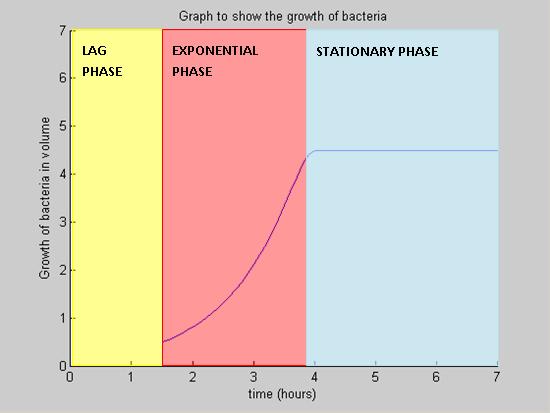
During the lag phase, the rate of growth is slow due to two main reasons, B. subtilis is absorbing nutrients in the medium and the replication machinery is being switched on. The higher the concentration of nutrients in the medium, the faster the rate of bacteria growth.
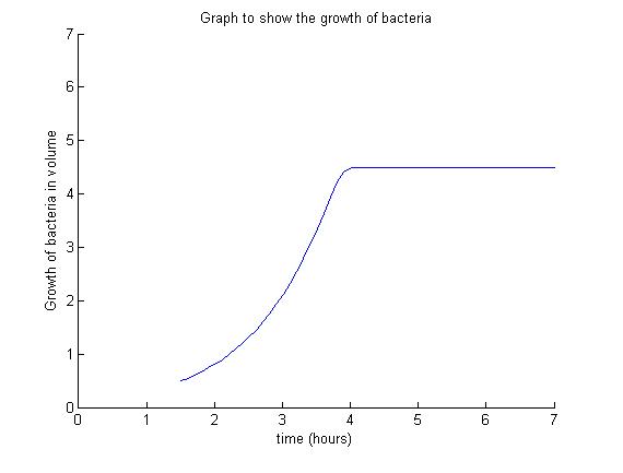
As a result, the volume of the bacteria increases, followed by an increase in the number of bacteria.
Exponential Phase
Both colony number and cell volume increase exponentially during this phase. Our model assumes concentration of the nutrients inside the bacteria is constant.
Stationary Phase
The growth of the colony ceases in number and in volume due to a finite concentration of nutrients, hence it does not have a gradient. Other causes may be death and cell division.
According to the model, the maximum growth of the bacteria is determined by the concentration of nutrients available initially.
To further enhance the accuracy of the model, the following information will be extracted from experimental data:
- Time span of lag phase, stationary phase and exponential phase
- The growth rate
|
|
| Results
|
|
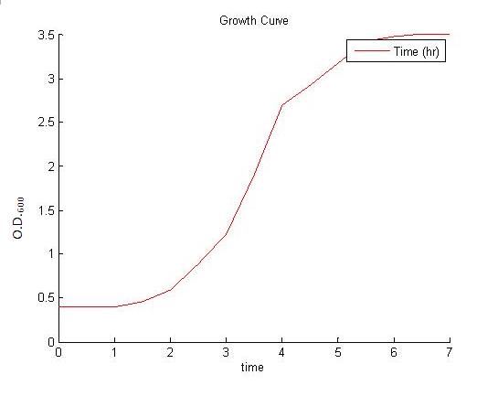
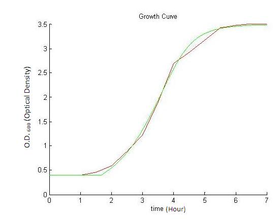
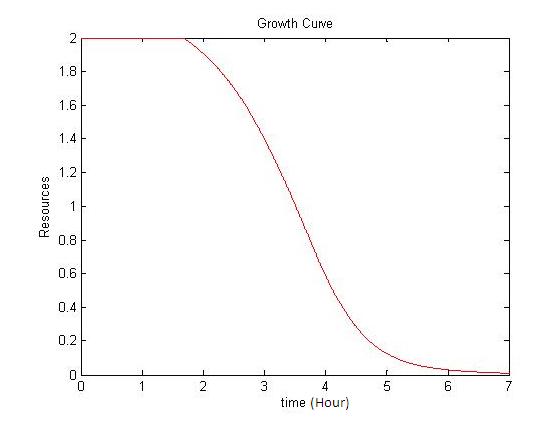
The model for the growth curve was fitted to the experimental results as shown below. The experimental results is depicted by the red curve, while our model is shown by the green curve. The resource curve was also plotted as a function of time and is shown below. Based on our experimental results from the Wet Lab, a log graph was plotted to determine the growth rate. The growth rate was then determined from the gradient of the log graph. This value was included when simulating the growth model using MATLAB.
|
|
|
| | Experimental Results
| Fitted Curve
| Resource Curve
|
The following constants used to generate the model were found to yield the best fit to experimental results.
GROWTH CONSTANT (A): 1.3494
INITIAL NUTRIENT CONCENTRATION (R0): 2
HILL COEFFICIENT (n): 1.25
INITIAL OD: 0.4
CONSTANT (<math>\alpha</math>): 0.64516
|
|
| The Model
|
|
The model illustrates the main growth phases the B. subtilis undergoes. These are identified as the lag phase, the exponential phase and the stationary phase. The death phase is a constitutive event and it is possible that it exerts an influence on the three phases discussed below. However, to simplify a complicated model, it is less relevant in this case and therefore is not included in this model.
The M-file used to generate the model below is located in the Appendices section of the Dry Lab hub.
 
|
|
|
 "
"


