Team:NTU-Singapore/Modelling/Stochastic Modeling
From 2008.igem.org
Lalala8585 (Talk | contribs) |
Lalala8585 (Talk | contribs) (→Detection & Lysis System Version 2) |
||
| (10 intermediate revisions not shown) | |||
| Line 22: | Line 22: | ||
=='''Stochastic Model For E7 + Imm Production'''== | =='''Stochastic Model For E7 + Imm Production'''== | ||
| - | [[Image:Sys1.JPG|600px|thumb|center|Cellware E7 | + | [[Image:Sys1.JPG|600px|thumb|center|Cellware E7 Production System]]<br> |
The above image shows the model that was used in Cellware for the 1st System. <br> | The above image shows the model that was used in Cellware for the 1st System. <br> | ||
The Purple Rectangles represent the DNA.<br> | The Purple Rectangles represent the DNA.<br> | ||
| Line 55: | Line 55: | ||
'''Gillespie Model''' | '''Gillespie Model''' | ||
The stochastic modeling results are as shown and a total of 10 runs was done. The results are also compared to the Deterministic Modeling Output. One might then think that since the Deterministic Models produce results in concentrations while the Stochastic Models give their results in the number of molecules, the results are not actually the same. That is perfectly true. The reason for putting the results together is for a simple visualisation of the results. Again, it is stressed that the behaviour of the models are of greater importance, not the numerical values.<br> | The stochastic modeling results are as shown and a total of 10 runs was done. The results are also compared to the Deterministic Modeling Output. One might then think that since the Deterministic Models produce results in concentrations while the Stochastic Models give their results in the number of molecules, the results are not actually the same. That is perfectly true. The reason for putting the results together is for a simple visualisation of the results. Again, it is stressed that the behaviour of the models are of greater importance, not the numerical values.<br> | ||
| - | [[Image:Sys1_gillespie.jpg||center|thumb|800px|Cellware Gillespie model | + | [[Image:Sys1_gillespie.jpg||center|thumb|800px|Cellware Gillespie model: E7 production system]]<br> |
The run was done with 10mM lactose induction. As seen, the model is simple and the stochastic model produces results that are close to the deterministic model. | The run was done with 10mM lactose induction. As seen, the model is simple and the stochastic model produces results that are close to the deterministic model. | ||
'''Gibson Next Reaction Method''' | '''Gibson Next Reaction Method''' | ||
| - | [[Image:Sys1_gibson.jpg|center|thumb|800px|Cellware Gibson Next Reaction method | + | [[Image:Sys1_gibson.jpg|center|thumb|800px|Cellware Gibson Next Reaction method: E7 production system]]<br> |
| - | =='''Stochastic Model For Lysis Production'''== | + | =='''Stochastic Model For Detection & Lysis Production System'''== |
| - | ===''' | + | ==='''Detection & Lysis System Version 1'''=== |
| - | [[Image:Lysis_new_diag2.JPG|thumb|center|700px|Cellware Models | + | [[Image:Lysis_new_diag2.JPG|thumb|center|700px|Cellware Models: Detection & Lysis Production System Version 1]]<br> |
| - | As discussed before[https://2008.igem.org/Team:NTU-Singapore/Modelling/Deterministic_Modeling#New_Lysis_Production_System | + | As discussed before in [https://2008.igem.org/Team:NTU-Singapore/Modelling/Deterministic_Modeling#New_Lysis_Production_System deterministic modeling section], a Detection & Lysis System Version 1 was introduced and a model was built to see how the results would turn out. |
| - | [[Image:Gip_new_lysis_onerun.jpg|800px|thumb|center|Cellware Gillespie model | + | [[Image:Gip_new_lysis_onerun.jpg|800px|thumb|center|Cellware Gillespie model: Detection & Lysis System Version 1 (Single Run)]]<br> |
| - | [[Image:Gip_new_lysis.jpg|800px|thumb|center|Cellware Gillespie model | + | [[Image:Gip_new_lysis.jpg|800px|thumb|center|Cellware Gillespie model: Detection & Lysis System Version 2]]<br> |
| - | As | + | As observed, the Detection & Lysis production System Version 1 was modeled using the Gillespie model. After 10 runs, results indicated that the Lysis protein production would tend to a steady state after some time. |
| - | ===''' | + | ==='''Detection & Lysis System Version 2'''=== |
| - | [[Image:Sys2.JPG|center|thumb|600px|Cellware model | + | [[Image:Sys2.JPG|center|thumb|600px|Cellware model: Detection & Lysis Production System Version 2]]<br> |
| - | The above diagram shows how we have modeled the Lysis Production system in Cellware. Again the legend is the same as the first E7 production system. We would also like to see how the Deterministic models turn out. The results are as shown.<br> | + | The above diagram shows how we have modeled the Detection & Lysis Production system Version 2 (with biological AND gate) in Cellware. Again the legend is the same as the first E7 production system. We would also like to see how the Deterministic models turn out. The results are as shown.<br> |
<center> | <center> | ||
{| align="center" border="1" | {| align="center" border="1" | ||
| Line 112: | Line 112: | ||
|} | |} | ||
</center> | </center> | ||
| - | [[Image:Sys2_DetMod.jpg|center|thumb|700px|Cellware Lysis Production System | + | [[Image:Sys2_DetMod.jpg|center|thumb|700px|Cellware Deterministic Model: Detection & Lysis Production System Version 2]]<br> |
As we can see, a very similar outcome is observed as compared to the [https://2008.igem.org/Team:NTU-Singapore/Modelling/Deterministic_Modeling#Lysis_Production_system model] we had obtained in Simulink. The difference in the Lysis protein output under the conditions that Ai-2 is present alone and when Iron and Ai-2 is present is not very pronounced. | As we can see, a very similar outcome is observed as compared to the [https://2008.igem.org/Team:NTU-Singapore/Modelling/Deterministic_Modeling#Lysis_Production_system model] we had obtained in Simulink. The difference in the Lysis protein output under the conditions that Ai-2 is present alone and when Iron and Ai-2 is present is not very pronounced. | ||
'''Gillespie Model''' | '''Gillespie Model''' | ||
For the Stochastic model, the number of molecules are also a guess and more work has to be done is refining the parameters. Presented here is the initial results for the condition that both Ai-2 and iron ions are present, thereby activating the and gate. The stochastic model results are also compared with the deterministic model. | For the Stochastic model, the number of molecules are also a guess and more work has to be done is refining the parameters. Presented here is the initial results for the condition that both Ai-2 and iron ions are present, thereby activating the and gate. The stochastic model results are also compared with the deterministic model. | ||
<br> | <br> | ||
| - | [[Image:Sys2_gillespie.jpg|center|thumb|800px|Cellware Gillespie model | + | [[Image:Sys2_gillespie.jpg|center|thumb|800px|Cellware Gillespie model: Detection & Lysis production system Version 2 ]]<br> |
A total of 10 runs was done to observe the results. As expected, the random nature of the algorithm will give unique results for each run. Although the variations here are much larger compared to the first system, the general trend is still similar.<br> | A total of 10 runs was done to observe the results. As expected, the random nature of the algorithm will give unique results for each run. Although the variations here are much larger compared to the first system, the general trend is still similar.<br> | ||
'''Gibson Next Reaction Method''' | '''Gibson Next Reaction Method''' | ||
| - | [[Image:Sys2_gibson.jpg|center|thumb|800px|Cellware Gibson Next Reaction Method | + | [[Image:Sys2_gibson.jpg|center|thumb|800px|Cellware Gibson Next Reaction Method: Detection & Lysis Production System Version 2]]<br> |
'''Hybrid Model''' | '''Hybrid Model''' | ||
A run using the Hybrid Stochastic ODE solver was also done just to see how the results would vary. The model's basis is to introduce noise elements into the deterministic model and the solvers employ both deterministic ODE solvers and stochastic solvers. The result is as shown. | A run using the Hybrid Stochastic ODE solver was also done just to see how the results would vary. The model's basis is to introduce noise elements into the deterministic model and the solvers employ both deterministic ODE solvers and stochastic solvers. The result is as shown. | ||
| - | [[Image:Sys2_Hyb.jpg|center|thumb|800px|Cellware Hybrid model | + | [[Image:Sys2_Hyb.jpg|center|thumb|800px|Cellware Hybrid model: Detection & Lysis Production System Version 2]]<br> |
A total of 3 runs using the Hybrid ODE solver was done and the outputs were put together with the Deterministic Model for easy comaprison. The modeling results show the Hybrid model results don't vary much as they overlap one another. To fully appreciate the stochastic nature of the systems, the Gillispie Algorithm and other Stochastic Algorithms seem to be a better choice | A total of 3 runs using the Hybrid ODE solver was done and the outputs were put together with the Deterministic Model for easy comaprison. The modeling results show the Hybrid model results don't vary much as they overlap one another. To fully appreciate the stochastic nature of the systems, the Gillispie Algorithm and other Stochastic Algorithms seem to be a better choice | ||
| Line 131: | Line 131: | ||
| - | [[Image: | + | [[Image:Lysis_stoch_Compare2_copy.jpg||center|thumb|800px|Comparison of the 2 Detection & Lysis system]]<br> |
| - | For the sake of interest, we can see that the models also show that the Lysis | + | For the sake of interest, we can see that the models also show that the Detection & Lysis system with AND gate has a slower response time to the Version 1 system. The Version 1 system can achieve the faster lysis of the cell, but again, fails in specificity. |
=Updates= | =Updates= | ||
| - | Currently the Simulations for the Lysis | + | Currently the Simulations for the Detection & Lysis system tend to terminate prematurely at time = 70 min. The reason is still unknown but it could be due to the fact that the system is much more complicated than the E7 production system. Work is still being done to see if more models can be generated using Cellware. The program is generally easy to manipulate and the interface is quite user-friendly. If you have any comments on how our modeling exercise can be improved, don't hesitate to leave us an [mailto:ntu.igem@gmail.com email] |
. All contributions will be acknowledged by our team. | . All contributions will be acknowledged by our team. | ||
</div> | </div> | ||
| + | <br><br> | ||
| + | <html> | ||
| + | <script language=Javascript1.2> | ||
| + | <!-- | ||
| + | |||
| + | var tags_before_clock = "<b>It is now " | ||
| + | var tags_middle_clock = "on" | ||
| + | var tags_after_clock = "</b>" | ||
| + | |||
| + | if(navigator.appName == "Netscape") { | ||
| + | document.write('<layer id="clock"></layer><br>'); | ||
| + | } | ||
| + | |||
| + | if (navigator.appVersion.indexOf("MSIE") != -1){ | ||
| + | document.write('<span id="clock"></span>'); | ||
| + | } | ||
| + | |||
| + | DaysofWeek = new Array() | ||
| + | DaysofWeek[0]="Sunday" | ||
| + | DaysofWeek[1]="Monday" | ||
| + | DaysofWeek[2]="Tuesday" | ||
| + | DaysofWeek[3]="Wednesday" | ||
| + | DaysofWeek[4]="Thursday" | ||
| + | DaysofWeek[5]="Friday" | ||
| + | DaysofWeek[6]="Saturday" | ||
| + | |||
| + | Months = new Array() | ||
| + | Months[0]="January" | ||
| + | Months[1]="February" | ||
| + | Months[2]="March" | ||
| + | Months[3]="April" | ||
| + | Months[4]="May" | ||
| + | Months[5]="June" | ||
| + | Months[6]="July" | ||
| + | Months[7]="August" | ||
| + | Months[8]="September" | ||
| + | Months[9]="October" | ||
| + | Months[10]="November" | ||
| + | Months[11]="December" | ||
| + | |||
| + | function upclock(){ | ||
| + | var dte = new Date(); | ||
| + | var hrs = dte.getHours(); | ||
| + | var min = dte.getMinutes(); | ||
| + | var sec = dte.getSeconds(); | ||
| + | var day = DaysofWeek[dte.getDay()] | ||
| + | var date = dte.getDate() | ||
| + | var month = Months[dte.getMonth()] | ||
| + | var year = dte.getFullYear() | ||
| + | |||
| + | var col = ":"; | ||
| + | var spc = " "; | ||
| + | var com = ","; | ||
| + | var apm; | ||
| + | |||
| + | if (date == 1 || date == 21 || date == 31) | ||
| + | {ender = "<sup>st</sup>"} | ||
| + | else | ||
| + | if (date == 2 || date == 22) | ||
| + | {ender = "<sup>nd</sup>"} | ||
| + | else | ||
| + | if (date == 3 || date == 23) | ||
| + | {ender = "<sup>rd</sup>"} | ||
| + | |||
| + | else | ||
| + | {ender = "<sup>th</sup>"} | ||
| + | |||
| + | if (12 < hrs) { | ||
| + | apm="<font size='-1'>pm</font>"; | ||
| + | hrs-=12; | ||
| + | } | ||
| + | |||
| + | else { | ||
| + | apm="<font size='-1'>am</font>"; | ||
| + | } | ||
| + | |||
| + | if (hrs == 0) hrs=12; | ||
| + | if (hrs<=9) hrs="0"+hrs; | ||
| + | if (min<=9) min="0"+min; | ||
| + | if (sec<=9) sec="0"+sec; | ||
| + | |||
| + | if(navigator.appName == "Netscape") { | ||
| + | document.clock.document.write(tags_before_clock+hrs+col+min+col+sec+apm+spc+tags_middle_clock+spc+day+com+spc+date+ender+spc+month+com+spc+year+tags_after_clock); | ||
| + | document.clock.document.close(); | ||
| + | } | ||
| + | |||
| + | if (navigator.appVersion.indexOf("MSIE") != -1){ | ||
| + | clock.innerHTML = tags_before_clock+hrs+col+min+col+sec+apm+spc+tags_middle_clock+spc+day+com+spc+date+ender+spc+month+com+spc+year+tags_after_clock; | ||
| + | } | ||
| + | } | ||
| + | |||
| + | setInterval("upclock()",1000); | ||
| + | //--> | ||
| + | </script> | ||
| + | </html> | ||
Latest revision as of 00:29, 30 October 2008
|
Contents |
Stochastic Modeling
Preliminary Run
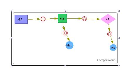
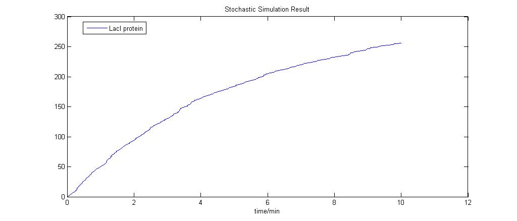
This model was generated using the program [http://www.cellware.org/index.html CellWare]. The above model was simulated using a Hybrid ODE solver that uses both deterministic and stochastic solvers. Work is now being done to see if this program can be used to build and simulate our systems.
All models below have been created using Cellware. [http://x.amath.unc.edu:16080/BioNetS/ Bionets2] is another option but we would first explore the use of the former program. The outputs are exported to MATLAB for plotting and visualisation.
Stochastic models using Gillispie Algorithm do not seem to work well as they seem to require a lot of computing power. Hybrid Stochastic ODEs seems to work better but the accuracy of the results seems to be compromised.
It is advised that the viewer observe the trends rather than the actual values given in the models. The modeling results would give us more of an idea of how the system would react rather than tell us exactly how much of a particular protein would be expressed. We hope that by doing this modeling exercise, we can learn more about our system.
Stochastic Model For E7 + Imm Production
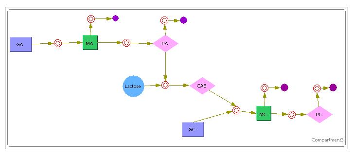
The above image shows the model that was used in Cellware for the 1st System.
The Purple Rectangles represent the DNA.
The Green Rectangles represent the mRNA.
The Pink Diamonds represent the Protein.
The Red Concentric Circles represent a certain reaction (Mass Action Reactions only, since its a requirement for Stochastic simulations)
The Purple Full Circles represented degradation of a particular substance.
Unlike the previous Simulink deterministic models, Cellware does not allow the user to inject certain variables at stipulated times. Therefore, the model shows inoculation of Lactose at the VERY START of the simulation. This is equivalent to exposing a newly divided cell to an environment of lactose rather than allowing it time to reach a certain steady state for its constitutive proteins. Nevertheless, we hope that the model can still allow us some insights into the system.
| Parameter | Deterministic(m/l) | Stochastic(No. of Molecules) |
| GA | 28 | 28 |
| GC | 28 | 28 |
| Lactose | 10 | 10 |
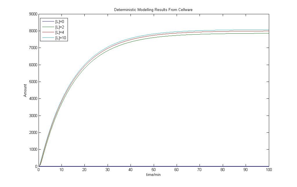
Before we actually use the program to run any form of stochastic simulations, it would be necessary to check how its deterministic models would turn out. By varying the amount of Lactose input, a few graphs were obtained and they are as shown.
The model shows that there are differences in the output when the Lactose is changed but they are not exactly significant. However the model still shows very similar behaviour to the model we had obtained using Simulink earlier.
Gillespie Model
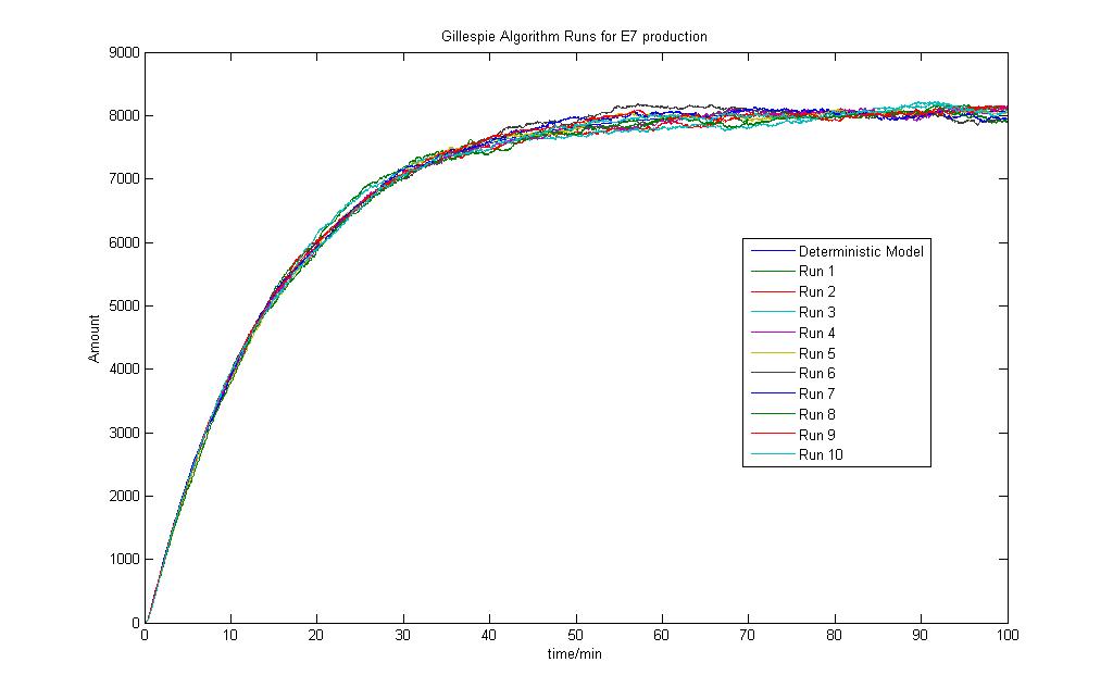
The stochastic modeling results are as shown and a total of 10 runs was done. The results are also compared to the Deterministic Modeling Output. One might then think that since the Deterministic Models produce results in concentrations while the Stochastic Models give their results in the number of molecules, the results are not actually the same. That is perfectly true. The reason for putting the results together is for a simple visualisation of the results. Again, it is stressed that the behaviour of the models are of greater importance, not the numerical values.
The run was done with 10mM lactose induction. As seen, the model is simple and the stochastic model produces results that are close to the deterministic model.
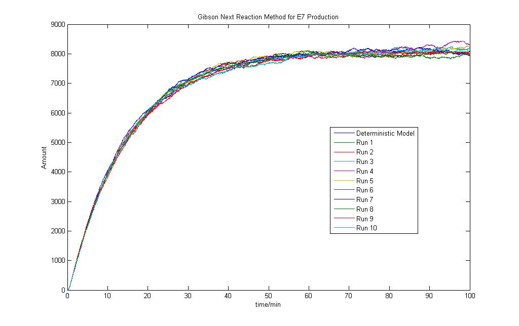
Gibson Next Reaction Method
Stochastic Model For Detection & Lysis Production System
Detection & Lysis System Version 1
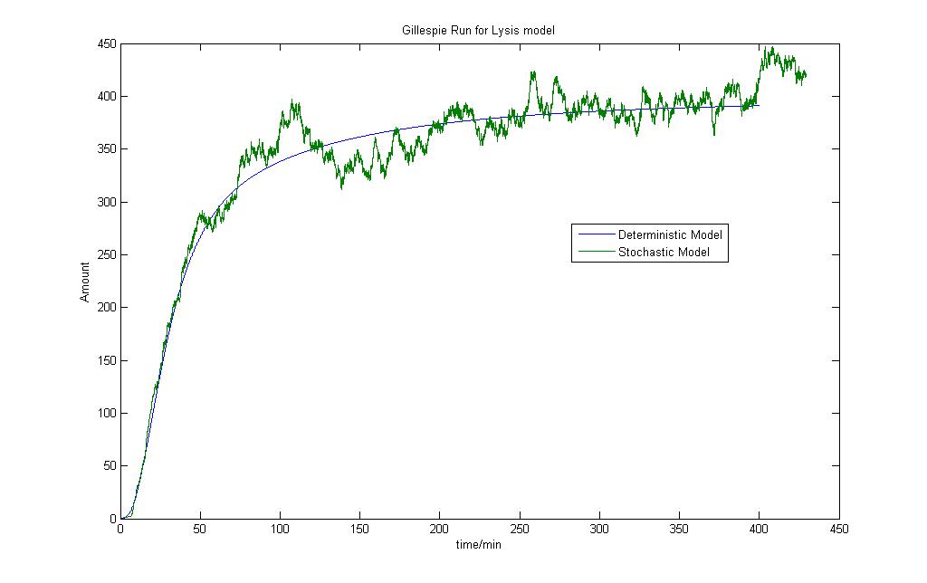
As discussed before in deterministic modeling section, a Detection & Lysis System Version 1 was introduced and a model was built to see how the results would turn out.
As observed, the Detection & Lysis production System Version 1 was modeled using the Gillespie model. After 10 runs, results indicated that the Lysis protein production would tend to a steady state after some time.
Detection & Lysis System Version 2
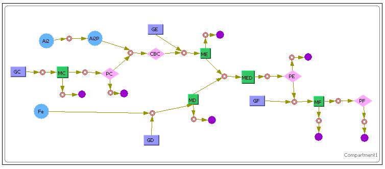
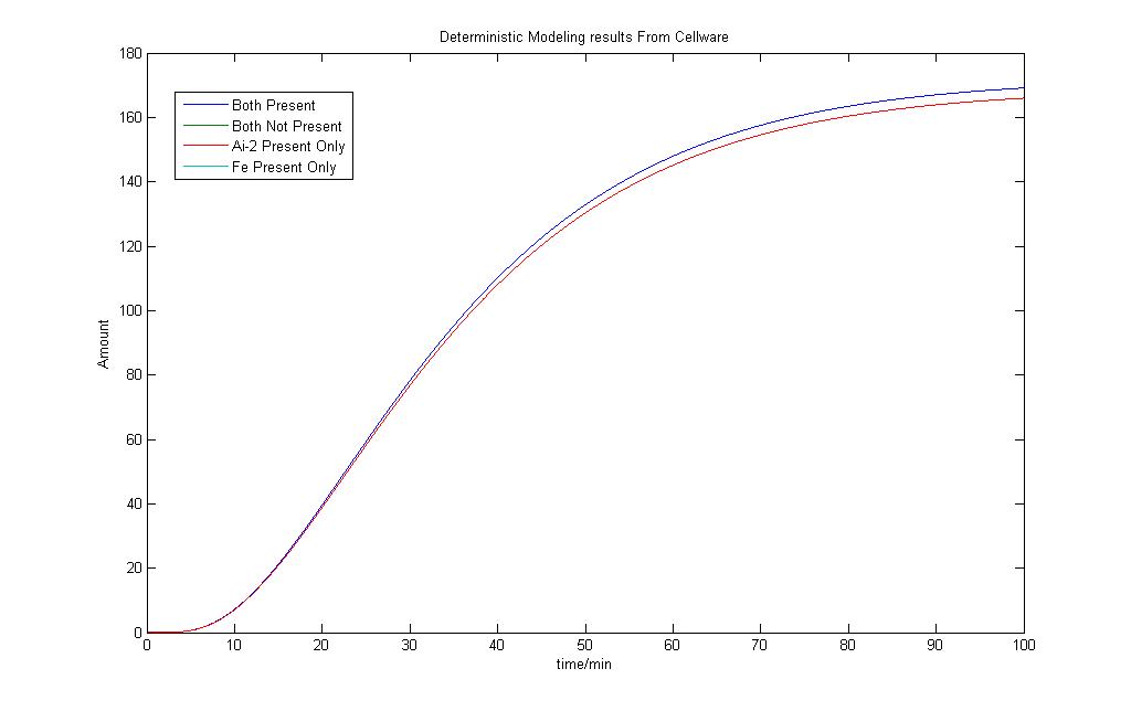
The above diagram shows how we have modeled the Detection & Lysis Production system Version 2 (with biological AND gate) in Cellware. Again the legend is the same as the first E7 production system. We would also like to see how the Deterministic models turn out. The results are as shown.
| Parameter | Deterministic(m/l) | Stochastic(No. of Molecules) |
| GC | 85 | 10 |
| GD | 85 | 10 |
| GE | 85 | 10 |
| GF | 85 | 10 |
| Ai-2(Present) | 238 | 28 |
| Ai-2(Not Present) | 0 | 0 |
| Fe(Present) | 130.05 | 15.3 |
| Fe (Not Present) | 127.5 | 15 |
As we can see, a very similar outcome is observed as compared to the model we had obtained in Simulink. The difference in the Lysis protein output under the conditions that Ai-2 is present alone and when Iron and Ai-2 is present is not very pronounced.
Gillespie Model
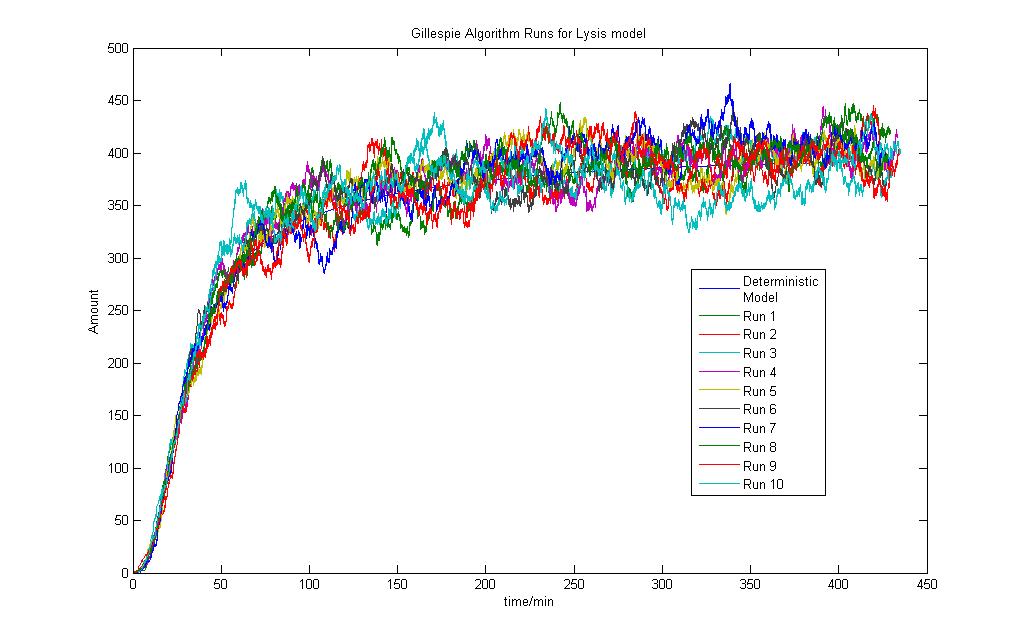
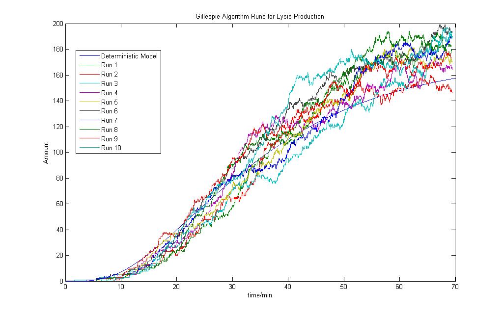
For the Stochastic model, the number of molecules are also a guess and more work has to be done is refining the parameters. Presented here is the initial results for the condition that both Ai-2 and iron ions are present, thereby activating the and gate. The stochastic model results are also compared with the deterministic model.
A total of 10 runs was done to observe the results. As expected, the random nature of the algorithm will give unique results for each run. Although the variations here are much larger compared to the first system, the general trend is still similar.
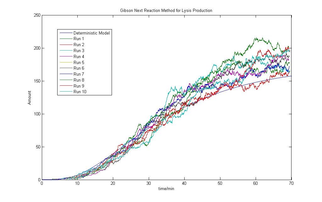
Gibson Next Reaction Method
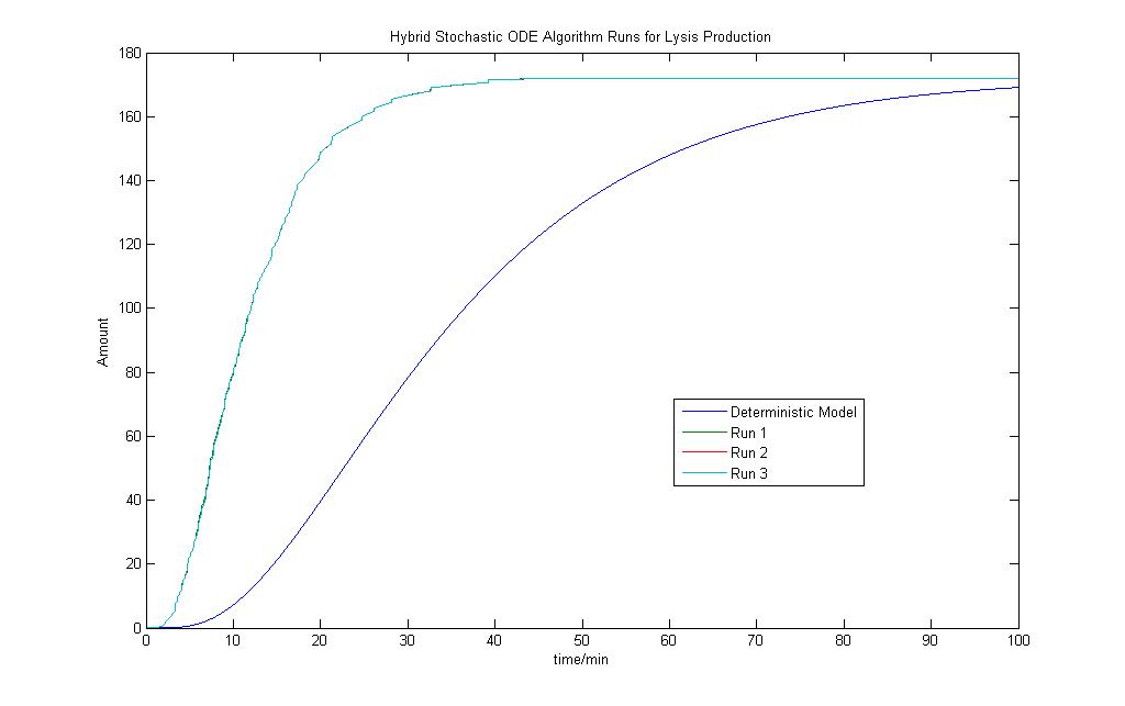
Hybrid Model A run using the Hybrid Stochastic ODE solver was also done just to see how the results would vary. The model's basis is to introduce noise elements into the deterministic model and the solvers employ both deterministic ODE solvers and stochastic solvers. The result is as shown.
A total of 3 runs using the Hybrid ODE solver was done and the outputs were put together with the Deterministic Model for easy comaprison. The modeling results show the Hybrid model results don't vary much as they overlap one another. To fully appreciate the stochastic nature of the systems, the Gillispie Algorithm and other Stochastic Algorithms seem to be a better choice
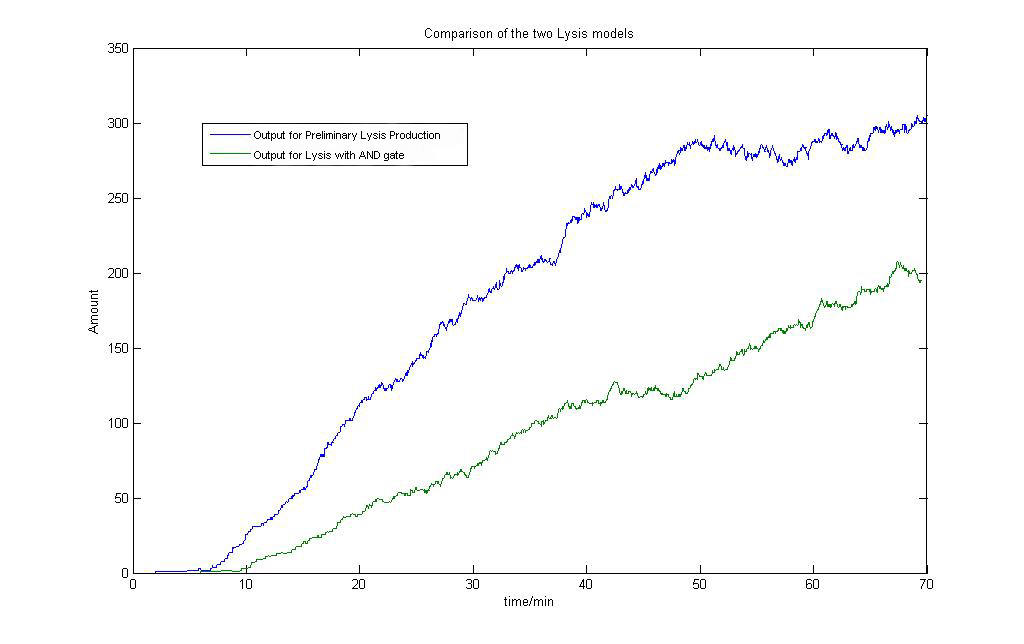
For the sake of interest, we can see that the models also show that the Detection & Lysis system with AND gate has a slower response time to the Version 1 system. The Version 1 system can achieve the faster lysis of the cell, but again, fails in specificity.
Updates
Currently the Simulations for the Detection & Lysis system tend to terminate prematurely at time = 70 min. The reason is still unknown but it could be due to the fact that the system is much more complicated than the E7 production system. Work is still being done to see if more models can be generated using Cellware. The program is generally easy to manipulate and the interface is quite user-friendly. If you have any comments on how our modeling exercise can be improved, don't hesitate to leave us an email . All contributions will be acknowledged by our team.
 "
"

