Team:EPF-Lausanne/Modeling
From 2008.igem.org
(→The Plan) |
|||
| Line 21: | Line 21: | ||
In order to solve these problems we will proceed in 3 steps: | In order to solve these problems we will proceed in 3 steps: | ||
| - | -Find the network exhibiting a transfer function corresponding to the rules displayed above without including the auto-sensing. | + | -Find the network exhibiting a transfer function, corresponding to the rules displayed above, without including the auto-sensing. |
| - | -Find out which species have to be co-expressed with the enzymes of the AHL signaling molecules in order to keep the same transfer function when the auto-sensing is included | + | -Find out which species have to be co-expressed with the enzymes of the AHL signaling molecules, in order to keep the same transfer function when the auto-sensing is included |
-Vary the model parameters in order to find a parameter set for which the switching between the two steady states can be achieved by giving perturbations only in the form of RHL signaling molecule gradients. | -Vary the model parameters in order to find a parameter set for which the switching between the two steady states can be achieved by giving perturbations only in the form of RHL signaling molecule gradients. | ||
Latest revision as of 22:15, 29 October 2008
| Home | The Team | The Project | Parts | 2-step PCR | Microfluidics | Modeling | Notebook |
|---|
Contents |
The Challenge...
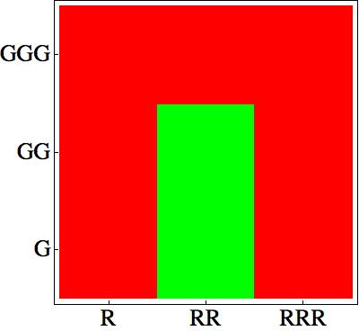
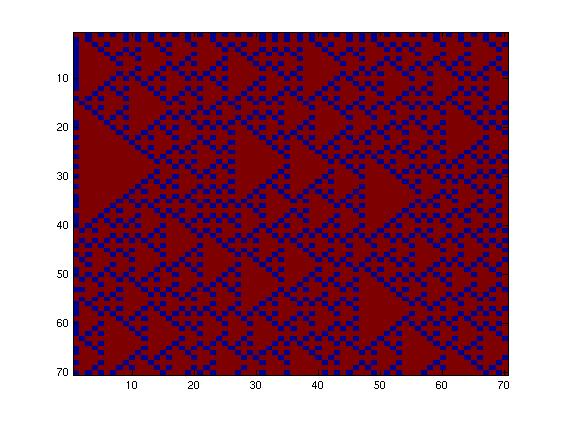
First of all, as described in the Project description, we choose some rules which give a nice pattern:
How can we design a genetic network corresponding to these rules?
The main challenge is to take into account that the cells sense their own AHL signaling molecules. As a consequence it is quite difficult to design a bistable network.
One solution is to co-express certain proteins, under the same promoter as the enzymes of the AHL signaling molecules (LuxI and RhlI).
Furthermore it should be possible to pass from one steady state to the other, by applying AHL concentration gradients to the cells. This is required in order to allow cells to change the state of their neighbors.
The Plan
In order to solve these problems we will proceed in 3 steps:
-Find the network exhibiting a transfer function, corresponding to the rules displayed above, without including the auto-sensing.
-Find out which species have to be co-expressed with the enzymes of the AHL signaling molecules, in order to keep the same transfer function when the auto-sensing is included
-Vary the model parameters in order to find a parameter set for which the switching between the two steady states can be achieved by giving perturbations only in the form of RHL signaling molecule gradients.
Double input model: auto-sensing is ignored
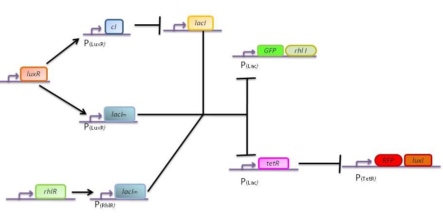
Here we describe a semi-quantitative model of the Lux band-pass detector and the Rhl high-pass detector. The model describes each proteins and sending molecules involved in the system. The feedback of the production of AHL signaling molecules inside the cell is ignored. At this stage, we test the ability of the system to process a constant input of green or red (ALux or ARhl) and choose an output state, either red or green.
States
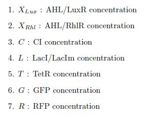
ODEs
Parameters
Simulation
The model nicely shows that for a certain range of AHL concentrations, the system can turn into either green or red. the following figure shows that we can achieve the band-pass filter on the red input and a high pass on the green input. Therefore, we can generate the choosen rule set where only medium level of red (AHL Lux) and low to medium level of green (AHL Rhl) can turn the system into the green state.
Bistable switch model
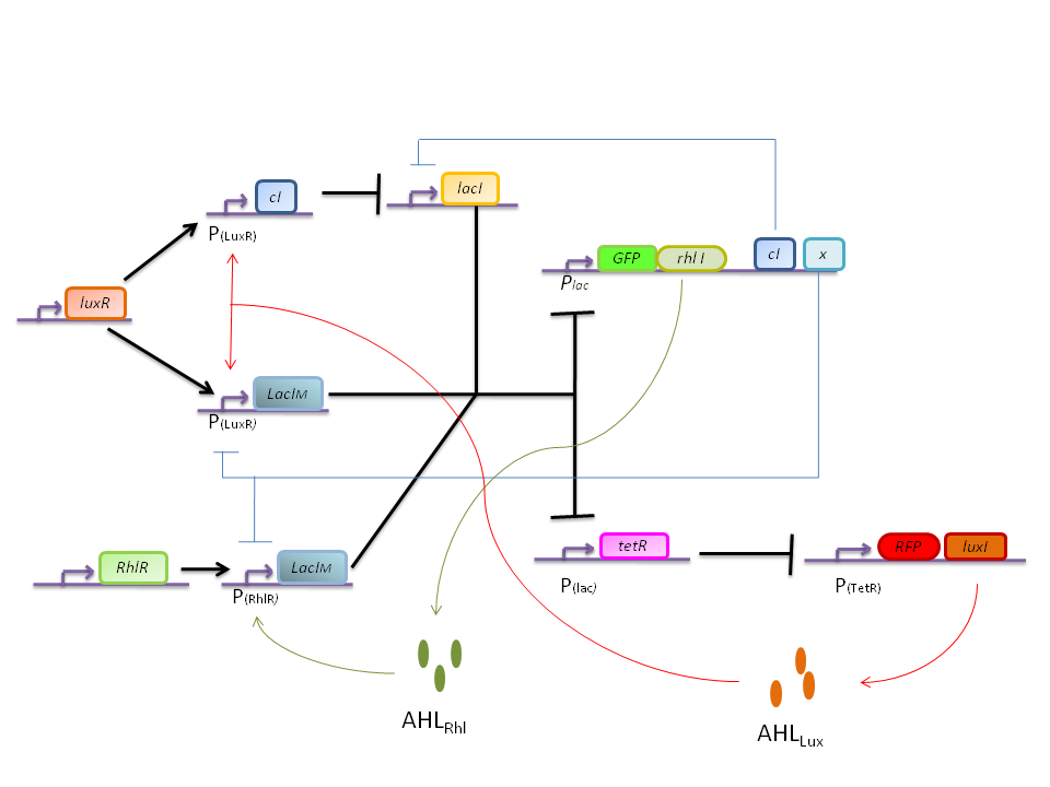
In this more complex model, we implemented the making of LuxI and RhlI in the cell, resulting in the self-production of AHL. We added two negative feedback loops (M and cI, blue arrows) that must help the system to lock itself into the green state. The red state is more stable than the green state and did not need any feedback to lock itself.
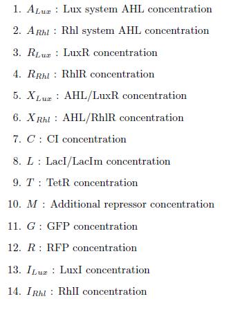
States
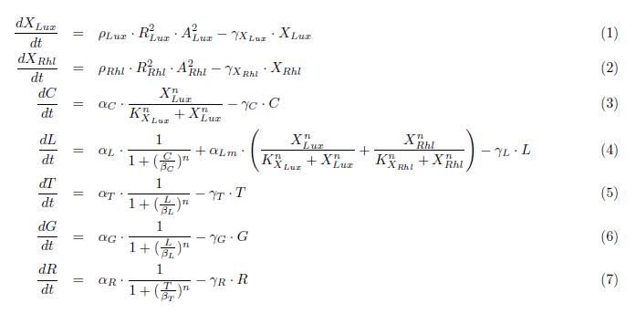
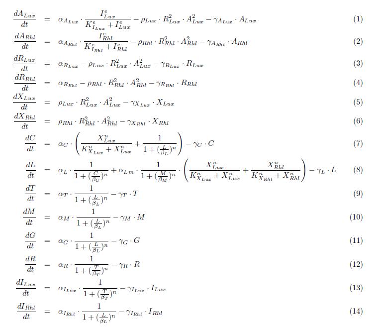
ODEs
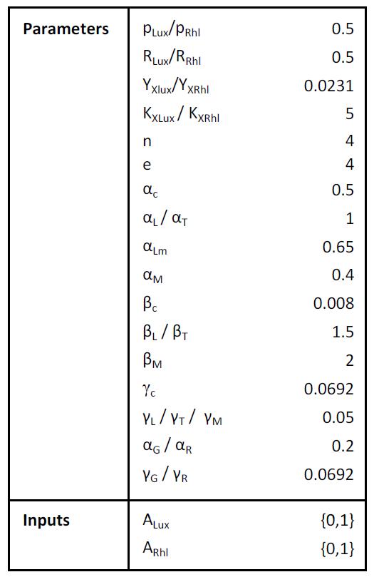
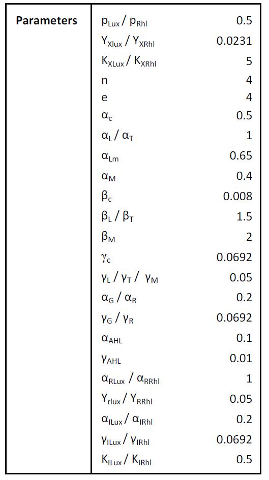
Parameters
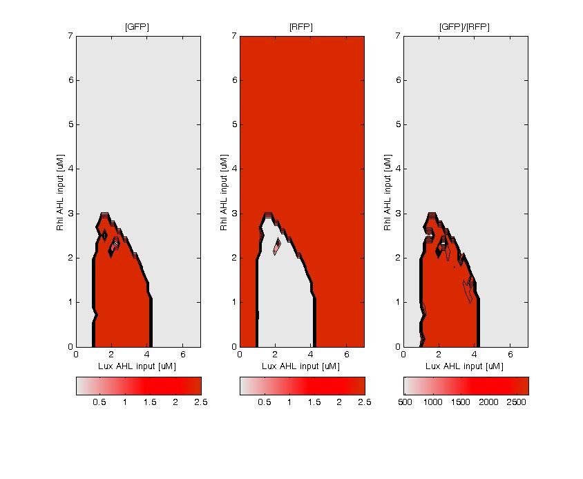
Simulation
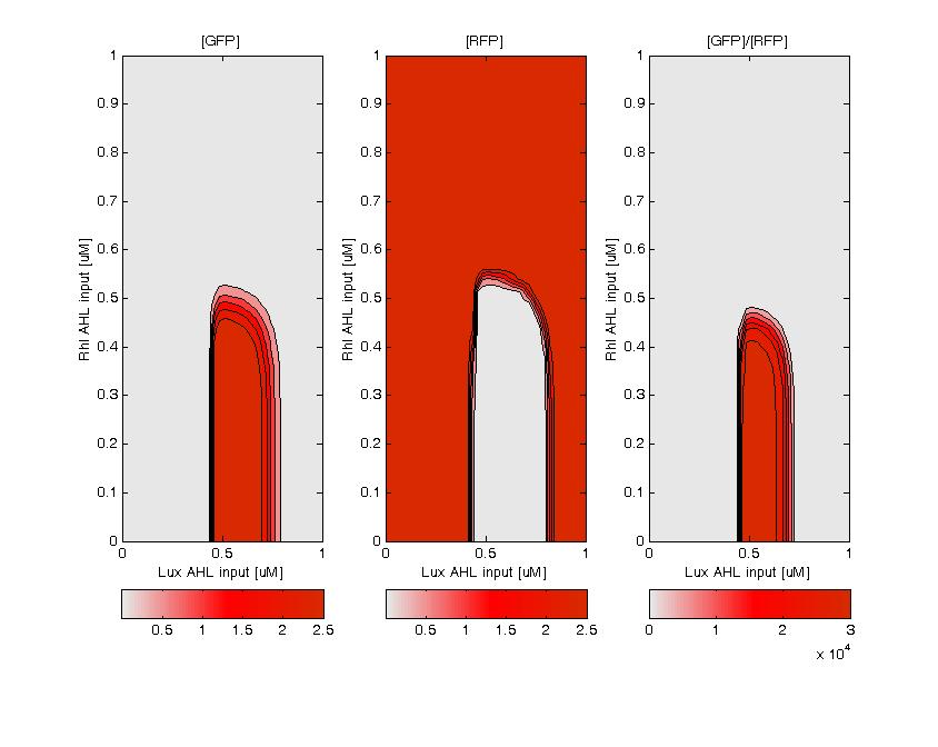
GFP (left) and RFP (middle) expression for concentration of AHL (Lux or Rhl) pulses. On the right, figure shows the ratio of GFP/RFP. This results shows that a given range of AHL can produce the green state. This is in good agreement with the rule set that we propose, where only medium level of red input (AHL Lux) and low to medium level of green input (AHL Rhl) can generate green.
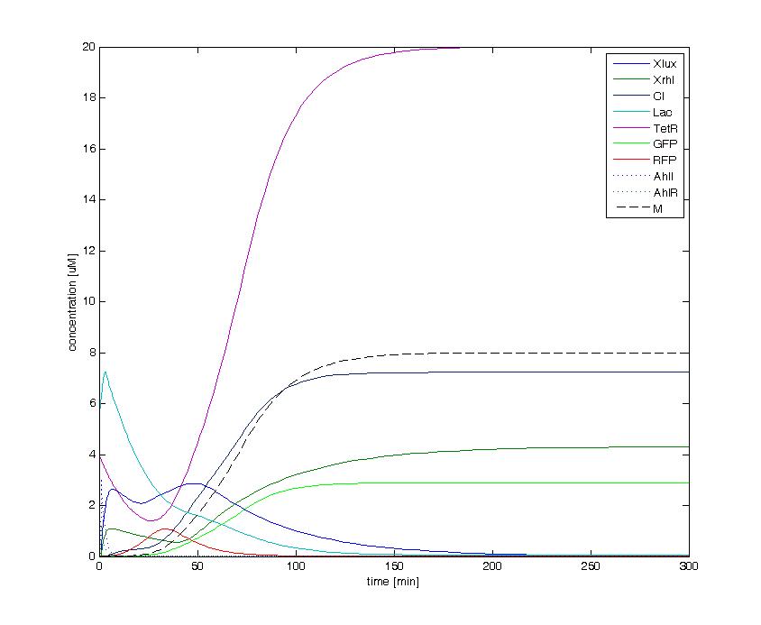
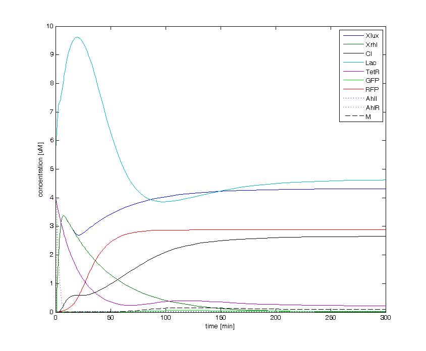
The following figures show the dynamics of the different states involved in the system for different AHL pulses. On the left, the system is locked into the green state after a pulse of 1.6 uM of Lux AHL and 3 uM of Rhl AHL. On the right, the system is locked into the red state after a pulse of 4 uM of Lux AHL and 4 uM of Rhl AHL. The model nicely shows the dominance of either TetR (purple line) or LacI (light blue line) for the green, respectively red state. It also shows the importance of the twos negative feedback made by the M represssor (dashed line) and cI (black line) to maintain the system in the green state.
Perturbation
One problem now, is that if we start from the green steady state it is not possible to perturb the system with only AHL pulses to pass to the red steady state, while the inverse is possible. Instead with perturbations on TetR and cI it is possible to make a red to green transition. But in our system a cell cannot perturb its neighbors in this way.
If we can force all the cells to be in the green state at the beginning of the experiment it should still be possible to have the generation of a pattern since the green to red transition can be achieved with an AHL pulse.
Still it would be much more interesting to have the other transition also allowed.
Is it possible to find other parameter sets where the green to red and red to green transitions can be achieved with AHL pulses?
Looking for the right parameters
Overview of the Genetic Algorithm
Exploring thoroughly a parameter space of dimension 23 is not an easy task and needs some advanced tools.
To tackle this problem we wrote a Genetic Algorithm in Mathematica language. Basically to use a genetic algorithm, two things are needed: a population and a fitness function. The fitness function assigns a value to an individuum of the population to quantify how good it performs.
In our problem the population consists of n parameter sets. Where n is typically big enough to sample efficiently the parameter space, but small enough to keep the computation time of the algorithm low. The fitness function is the crucial point of the algorithm (more about it in the next subsection).
The algorithm begins with the generation of an initial population.
Specifically for our needs we created a list of parameters called Boundaries in our program, where the parameters can be given in two ways:
-an upper and a lower boundary can be specified if we want the algorithm to look for this parameter within these boundaries.
-a single value can be given if we want the algorithm to keep this parameter constant.
This is useful if we can identify parameters that will not influence significantly the nature of the solution: for instance the degradation rates of the fluorescent reporter proteins. The parameter space to explore will thus be reduced without getting rid of the potentially interesting solutions.
A fitness is assigned to each individuum of the population.
If elitism is used the best performing individuum will be taken in the next generation. With a certain mutation probability, an individuum is taken at random with a probability proportional to its relative fitness and it is taken to the next generation with one of its parameters mutated. Otherwise two different parameter sets are selected from the population with probabilities proportional to their fitnesses and the mean of their parameters represent another individuum of the next generation.
These selections go on until the size of the next generation has reached the size as the initial population.
This process is iterated m times.
The fitness function
To say how good a parameter set is, first we define a function which corresponds to the expected behaviour of the transfer function. Then the ODE system with production of AHL molecules is simulated to reach the red steady state. From this steady state the system is simulated subjected to different AHL pulses. These pulses cover the different areas of the transfer function. To test whether the parameter set was a good candidate or not the inverse of the sum of the squared differences between the points from the simulated ODE and the points from the expected transfer function is taken.
If this value is high we have a good solution.
Results
Unfortunately the algorithm did not perform well and after a 1000 generations no parameter set with the expected property, to enable a red to green transition with an AHL pulse, was found.
Nevertheless this algorithm is a tool which can be useful to explore parameter sets for a given network model.
Possibly no such solution exists for this particular network. The problem is apparently that the red state is too stable.
Modifications that we could add are other co-expressed proteins with the enzymes of the AHL molecules.
 "
"
