|
|
| Line 58: |
Line 58: |
| | | | |
| | {{Imperial/Box1|Results| | | {{Imperial/Box1|Results| |
| | + | |
| | + | During our project, we mainly focused on obtaining the flagellar force, which is associated with the parameter A. <br> |
| | During the model fitting process, we modelled the motility of ''B. subtilis'' to have a maximum of two runs. Modelling the a cell with only a single run is relatively straightforward as it only generates a single set of parameters. When modelling a cell with two runs, we keep the value of parameter alpha constant since it is a ratio of the viscosity to the mass. We then let the final velocity of the cell's first run to be equal to parameter ''B'' the initial velocity of the cell's second run. The parameter which is allowed to change is parameter ''A'', the ratio of flagellar force to viscosity of the medium. | | During the model fitting process, we modelled the motility of ''B. subtilis'' to have a maximum of two runs. Modelling the a cell with only a single run is relatively straightforward as it only generates a single set of parameters. When modelling a cell with two runs, we keep the value of parameter alpha constant since it is a ratio of the viscosity to the mass. We then let the final velocity of the cell's first run to be equal to parameter ''B'' the initial velocity of the cell's second run. The parameter which is allowed to change is parameter ''A'', the ratio of flagellar force to viscosity of the medium. |
| | | | |
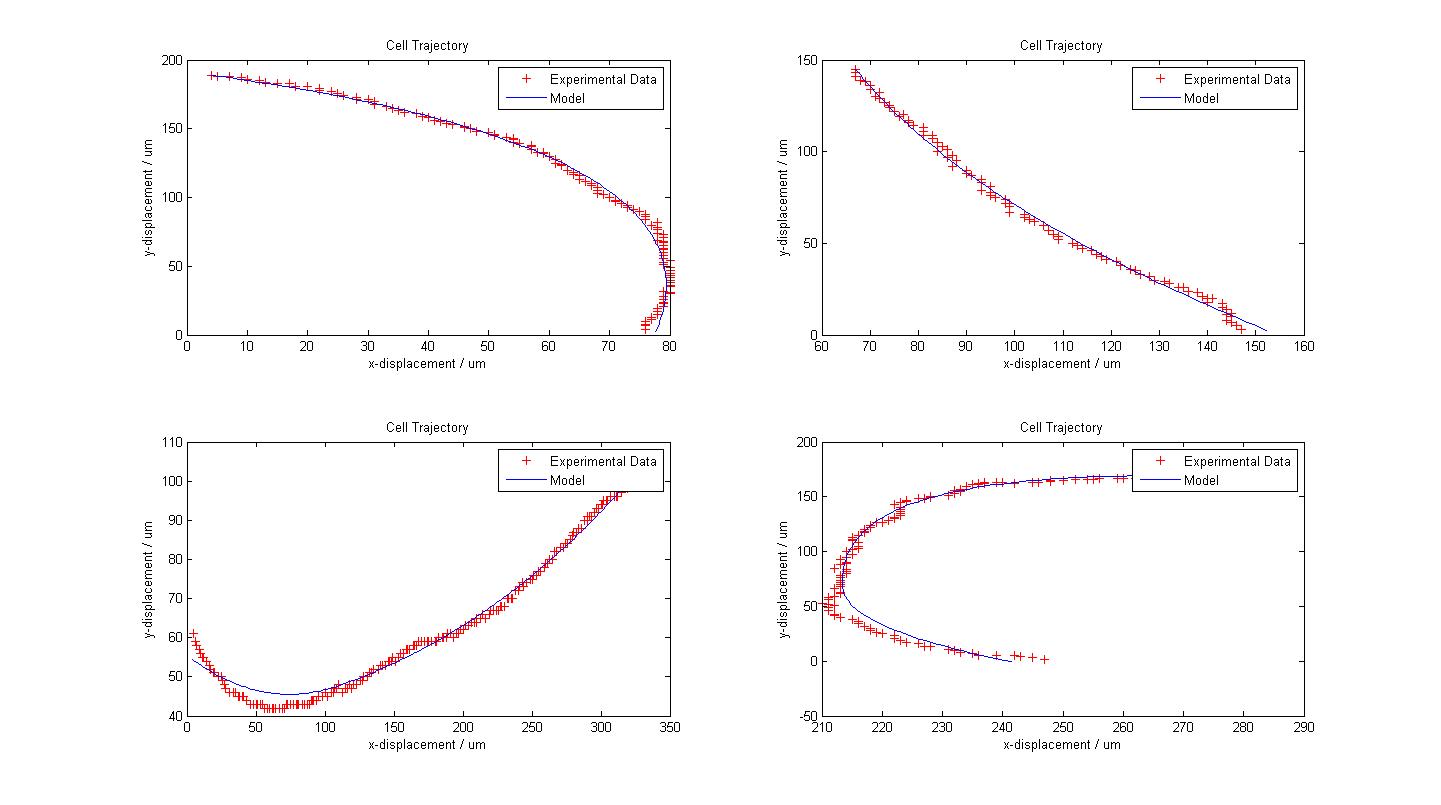
| - | The following figure shows the results of our model fitting. We have introduced a change in flagellar force at certain points of the cell trajectory so as to achieve a better fit. A maximum of two runs were allowed for each cell trajectory. | + | The following figure shows the results of our model fitting for few trajectories. We have introduced a change in flagellar force at certain points of the cell trajectory so as to achieve a better fit. A maximum of two runs were allowed for each cell trajectory. The results were good, sometimes surprisingly so. However, some results also suggest that a third or a fourth (short) change of flagellar force would help. <br> |
| | + | In general the choice of the change of flagellar force is a very complex problem. Automatic detection can certainly be developed but we lacked time to look into such solution. Instead we opted for the highly subjective manual detection of these changes |
| | + | |
| | | | |
| | {{{Pipe}} border{{Equals}}"0" cellpadding{{Equals}}"5" cellspacing{{Equals}}"0" align{{Equals}}"center" style{{Equals}}"background-color:transparent;color:#2B48B3;" | | {{{Pipe}} border{{Equals}}"0" cellpadding{{Equals}}"5" cellspacing{{Equals}}"0" align{{Equals}}"center" style{{Equals}}"background-color:transparent;color:#2B48B3;" |
| Line 70: |
Line 74: |
| | {{Pipe}}} | | {{Pipe}}} |
| | <br> | | <br> |
| - | The MATLAB Distribution Fitting Tool was used to model the distribution of parameter A. Parameter A was found to be exponentially distributed. The following figures describe the probability density function and cumulative density function. | + | |
| | + | The MATLAB Distribution Fitting Tool was used to model the distribution of the amplitude of parameter A. |
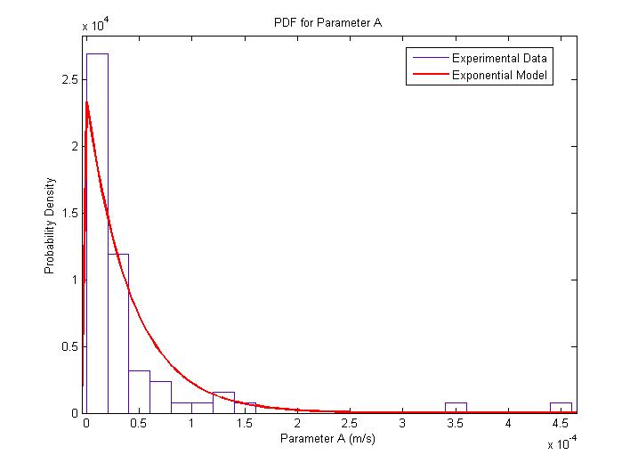
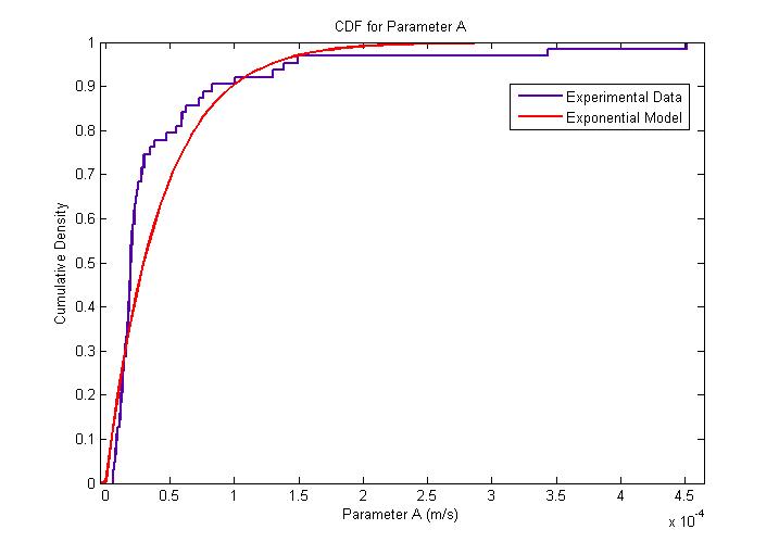
| | + | The amplitude of A is very interesting since it represents the velocity of the cell after a sufficiently long time has elapsed. The following figures describe the probability density function and cumulative density function. <br> |
| | + | The distribution was found to be close to an exponential distribution. This is rather surprising as we would have expected a Maxwell distribution instead. We think that this is due to the practical difficulty in determining with accuracy the changes of flagellar push and the consequent loss of accuracy in the extraction of the model parameters. |
| | + | |
| | | | |
| | {{{Pipe}} border{{Equals}}"0" cellpadding{{Equals}}"5" cellspacing{{Equals}}"0" align{{Equals}}"center" style{{Equals}}"background-color:transparent;color:#2B48B3;" | | {{{Pipe}} border{{Equals}}"0" cellpadding{{Equals}}"5" cellspacing{{Equals}}"0" align{{Equals}}"center" style{{Equals}}"background-color:transparent;color:#2B48B3;" |
|
Motility Analysis
| Approach
|
|
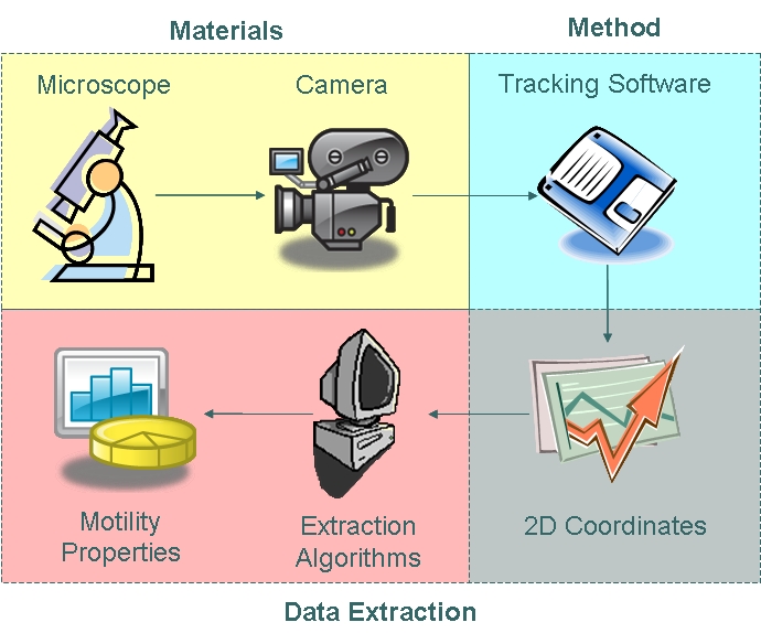
As part of our chassis characterisation process, we have decided to model B. subtilis motility. In order to do this, the approach illustrated below was taken. The first phase of modelling involved data collection using microscopy techniques and cell tracking. Collected data were then analysed using algorithms which enabled us to extract distributions of parameters as defined in our model.
From Data Collection to Data Analysis
Materials
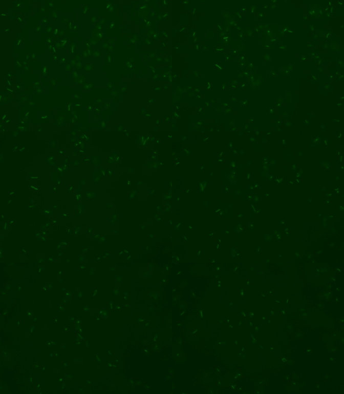
 Expression of GFP by Motile B.subtilis Expression of GFP by Motile B.subtilisWe used the Zeiss Axiovert 200 inverted microscope and Improvision Volocity acquisition software. This system offers a full incubation chamber with temperature control and a highly sensitive 1300x1000 pixel camera for fast low-light imaging. Video images are captured into memory by the system at a basal video frame rate of 16.3Hz. This can be further increased to 27.9Hz by performing x4 binning.
A short video of swimming B. subtilis is shown:
Method
In order to choose suitable tracking software, we generated a synthetic video and applied tracking algorithms to the data. We then assessed the reliability, validity and errors associated with the various tracking methods. We chose manual tracking as our method of tracking due to its high reliability and tolerable error.
>>> Details >>>
We manually tracked motile B. subtilis, obtaining two-dimensional coordinate data points which are described by the trajectory of the cells. The open source tracking software can be found here.
The coordinate data obtained were then fed into algorithms to model cell trajectory and motility. Algorithms used to extract motility data and fit cell trajectory data to models can be found in the appendices section.
|
|
| Motility Model
|
|
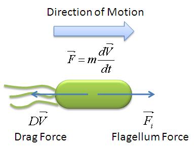
A simple mechanical model was developed by taking an analogy of B. subtilis propelled by its flagellum with that of a boat propelled by its motor. As the bacteria swims in the medium, it experiences two opposing forces: the flagellar force which propels it forward and drag force provided by the viscosity of the liquid medium. The drag force is analagous to friction which opposes the forward motion of objects on solid surfaces. The mechanical model is illustrated below:
Mechanical Model of Motile B.subtilis
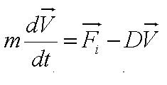
From the figure above, we equate the drag force and flagellar force to obtain:
Solving this first order ODE, we derive an expression for cell velocity:
 , where , where 
Solving the first order ODE for displacement, we derive an expression for cell trajectory:
Using our fitted data, we are able to determine parameters:
- Parameter A is the ratio of flagellar force to medium viscosity. It also represents the velocity of the cell after a sufficiently long time has elapsed, given that the flagellar force remains constant throughout its run.
- Parameter B is the initial cell velocity - in practice the velocity as we started to track the cell
- Parameter alpha is the ratio of the viscosity to the cell's mass.
As is widely known, the movement of bacteria is not that simple. Many bacteria have two distinct modes of movement: forward movement (swimming) and tumbling. The tumbling allows them to reorient and makes their movement a three-dimensional random walk.
But the boat-model can be used to analyze the swimming movement of bacteria with a few extra assumptions
- the medium is homogenous and the viscosity is constant throughout the medium
- The swimming movement is made of a finite number of trajectories that can be modelled with the boat-model. Such assumption corresponds to the idea that the bacterium pushes in a constant direction for a certain time and then pushes in a different direction for another time and so on.
- The movement of the bacteria is very smooth: there is continuity of the position and velocity
Given the random motion of bacteria, the outcome to such modelling will be the probability distribution of the model parameters and the time between the changes of pushes.
|
|
| Results
|
|
During our project, we mainly focused on obtaining the flagellar force, which is associated with the parameter A.
During the model fitting process, we modelled the motility of B. subtilis to have a maximum of two runs. Modelling the a cell with only a single run is relatively straightforward as it only generates a single set of parameters. When modelling a cell with two runs, we keep the value of parameter alpha constant since it is a ratio of the viscosity to the mass. We then let the final velocity of the cell's first run to be equal to parameter B the initial velocity of the cell's second run. The parameter which is allowed to change is parameter A, the ratio of flagellar force to viscosity of the medium.
The following figure shows the results of our model fitting for few trajectories. We have introduced a change in flagellar force at certain points of the cell trajectory so as to achieve a better fit. A maximum of two runs were allowed for each cell trajectory. The results were good, sometimes surprisingly so. However, some results also suggest that a third or a fourth (short) change of flagellar force would help.
In general the choice of the change of flagellar force is a very complex problem. Automatic detection can certainly be developed but we lacked time to look into such solution. Instead we opted for the highly subjective manual detection of these changes
|
|
| Fitted Models with Experimental Data from 4 Cells
|
The MATLAB Distribution Fitting Tool was used to model the distribution of the amplitude of parameter A.
The amplitude of A is very interesting since it represents the velocity of the cell after a sufficiently long time has elapsed. The following figures describe the probability density function and cumulative density function.
The distribution was found to be close to an exponential distribution. This is rather surprising as we would have expected a Maxwell distribution instead. We think that this is due to the practical difficulty in determining with accuracy the changes of flagellar push and the consequent loss of accuracy in the extraction of the model parameters.
|
|
|
| Probability Distribution for Parameter A
| Cumulative Distribution for Parameter A
|
|
|
| Conclusion
|
|
From our model fitting process, we can see that flagellar force is exponentially distributed. Our mechanical model though simple, fits the cell trajectory data extremely well as shown in the figure above. Further work would involve the use of a movable stage to track the movement of B. subtilis over its entire run, so as to obtain a distribution of other motility parameters associated with running and tumbling events.
|
|
|
 "
"

