Team:Michigan/Project/Modeling/Model1
From 2008.igem.org
(New page: __NOTOC__ {{Michigan Header}} {|class="wikitable" border="0" cellpadding="10" cellspacing="1" style="padding: 1px; background-color:dodgerblue; border: 1px solid mediumblue; text-align:...) |
|||
| Line 7: | Line 7: | ||
<font color=navy> | <font color=navy> | ||
| - | = '''<font color= | + | = '''<font color=royalblue size=6>Sequestillator Model 1: A simple model</font>''' = |
<div align='center'>[[Image:Model1Equations.png]] [[Image:Derivation.png]]</div> | <div align='center'>[[Image:Model1Equations.png]] [[Image:Derivation.png]]</div> | ||
Latest revision as of 02:43, 30 October 2008
|
|---|
|
Sequestillator Model 1: A simple modelParameters:
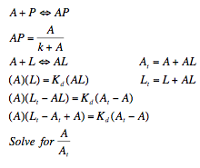
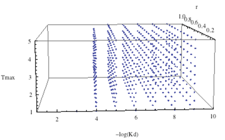
Professor Daniel Forger came up with this model for the Sequestillator. This simple system assumes the total amount of NifA in the system is constant, and considers three variable: NifL mRNA (mL), NifL (La), and a simple covalent modification of NifL (Lb). The quadratic mRNA production function comes from making rapid equilibrium assumptions (see box to the right of the equations. A= free unbound NifA, L = unbound NifL). From analyzing this small model, we were able to see that in order for oscillations to exist, there needed to be a tight binding between NifL and NifA (i.e., Kd is very small) and one-to-one titration of NifL and NifA (the mRNA production function = tmax*A/At, where A is free NifA in the system. A graph of the function vs. Lb is a oblique line).
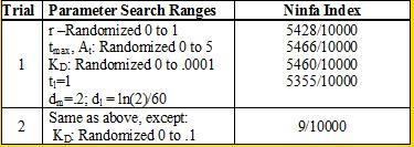
We see that if we increase our search range for the dissociation constant to 0 to .1, then we get a substantially smaller Ninfa index, illustrating the importance of having a tight binding between NifA and NifL.
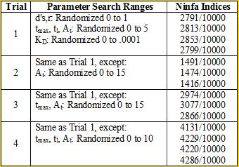
There was another aspect of our model that we can also verify: the importance of a one-to-one NifA/NifL titration: We see in trial 2, by increasing the range of At to 0 to 15 (and hence increasing the chance of having larger values of At), we have a reduction in the Ninfa index, as the system is unbalanced (too much At around). We return to similar Trial 1 results when we also vary tmax between 0 to 15 in Trial 3. FURTHER WORK THAT WILL BE PRESENTED DURING iGEM POSTER TALKS
|
|---|
 "
"


