Team:Imperial College/Growth Curve

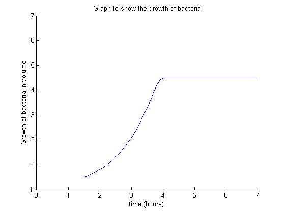
Part of our dry lab team concentrated on modelling the growth curve of B. subtilis. This is important to characterise the chassis; particularly, the growth of subtilis is a vital parameter for planning experiments for future projects. Characterisation increases the predictability of the growth of B. subtilis by determining, for example, its growth rate and the duration of its distinctive growth phases. In order to model the growth of B. subtilis, the process was broken down into three main steps, where a separate submodel is produced in MATLAB for each step. Each submodel is an ODE model, which can be simulated using MATLAB. The variables in each submodel can be adjusted according to the boundary conditions (from experimental results).

In the final step, a combination of Submodels 1 and 2 are superimposed with Submodel 3, resulting in a more complex model which enhances the accuracy of illustrating bacterial growth. For more details about the submodels, please see the Dry Lab Appendices page.

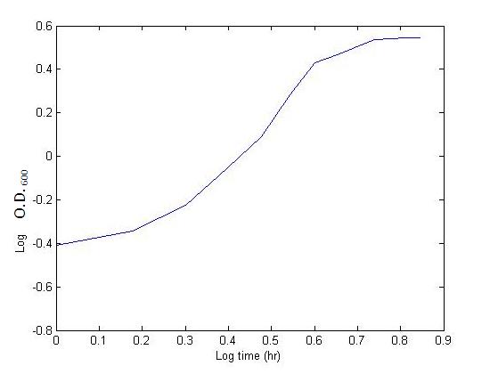
The graph on the right shows the log graph used to determine the growth rate.

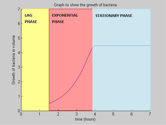
Lag Phase

During the lag phase, the rate of growth is slow. All nutrients are situated outside the cell initially. Some time is needed for an adequate amount of nutrients to move from the outside of the cell into the interior of the cell. This is vital as the cell requires the nutrients for growth.

Exponential Phase

Nutrients are consumed during the cell growth and the growth is exponential as long as there are enough nutrients available. The exchange of nutrients ensures that the intra- and extracellular nutrient concentration are the same.

Stationary Phase

The growth of the colony ceases in number and in volume due to a finite concentration of nutrients, hence it does not have a gradient. Other causes may be death and cell division.

To further enhance the accuracy of the model, the following information will be extracted from experimental data, resulting in a model that will produce a closer fit to the trend given by the experimental data.

• Time span of lag phase, stationary phase and exponential phase

• The growth rate

The model illustrates the main growth phases the B. subtilis undergoes. These are identified as the lag phase, the exponential phase and the stationary phase. The death phase is a constitutive event and it is possible that it exerts an influence on the three phases discussed below. However, to simplify a complicated model, it is less relevant in this case and therefore is not included in this model.

Advantage of looking at overall volume: we can to some extent overlook cell division: when a cell divides, we can assume the internal concentration of nutrients is almost instantly reset to the external concentration. During this time the total volume does not change

The M-file used to generate the model below is located in the Appendices section of the Dry Lab hub.

The model for the growth curve was fitted to the experimental results as shown below. The experimental results is depicted by the red curve, while our model is shown by the green curve. The resource curve was also plotted as a function of time and is shown below. Based on our experimental results from the Wet Lab, a log graph was plotted to determine the growth rate. The growth rate was then determined from the gradient of the log graph. This value was included when simulating the growth model using MATLAB.

Experimental Results	Fitted Curve	Resource Curve

The following constants used to generate the model were found to yield the best fit to experimental results:

GROWTH CONSTANT (A): 1.3494

INITIAL NUTRIENT CONCENTRATION (R₀): 2

HILL COEFFICIENT (n): 1.25

INITIAL OD: 0.4

CONSTANT (α): 0.64516

The model 'fit' is very good in exponential and stationary phases. However, this does not apply to the lag phase. This suggests that the model should be expanded in order to take into account phenomena such as the movement of the nutrients into the cells.