Team:NTU-Singapore/Parts/Parameter Estimation using Characterization Results
From 2008.igem.org
|
Contents |
Parameter Estimation
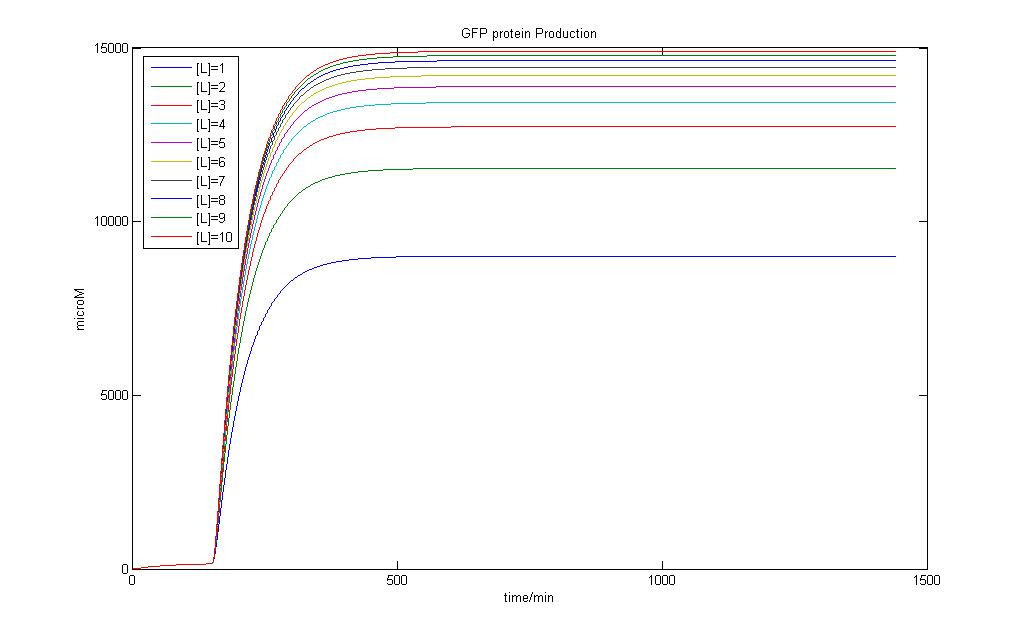
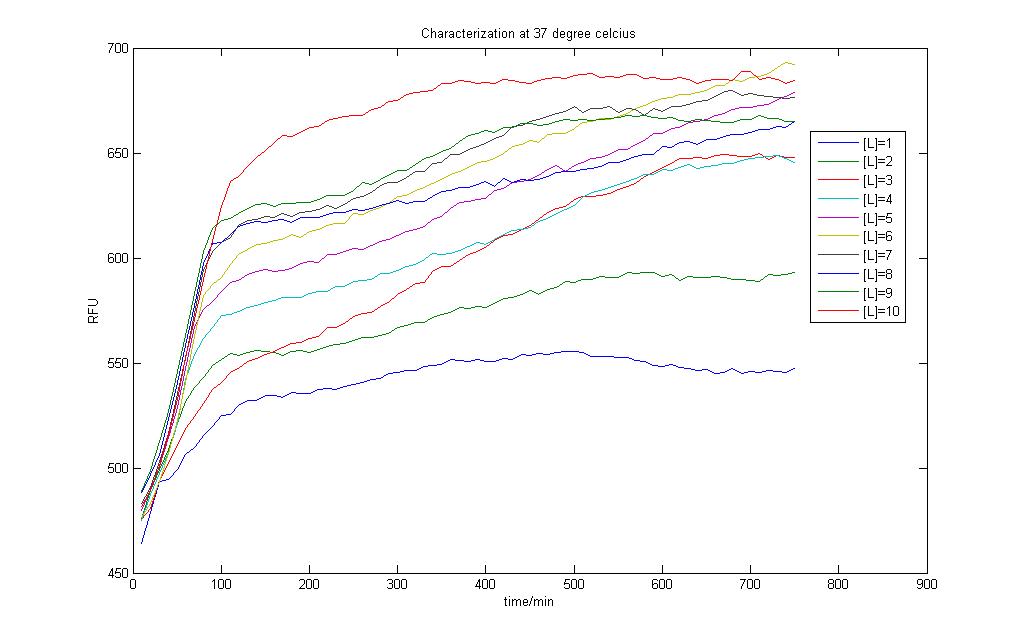
In the above two figures, we have a comparison between the model generated by our very own equations versus the RFU results that we have obtained using our characterization procedures. There are certain features that are our outstanding when these two figures are compared.
1)The deterministic model has not captured any of the stochastic features the real situation presented before us.
2)The model seems to hit steady state much faster than the actual situation
To test how the parameter estimation works out, we tried to input the RFU values as GFP protein produced, intrinsically assuming that both are directly proportional to one another. The results however are discouraging, prompting us to reconsider what went wrong. The results can be found in Failed Parameter Estimation Results link.
Careful observation of the results from the characterisation and one would notice that the output takes on the form of a sigmoid curve. Indeed, one of the major flaws in our modeling exercise was that the models don't account for cell growth. Even though we used M9 medium to do our characterisation, it is impossible to assume the cells don't multiply and grow within the 12 hour time period!
This prompts us to look into a better model such that we can first capture the essentials of the real situation before we decide to use our models with our characterisation results.
Creating a Logistic Growth Construct
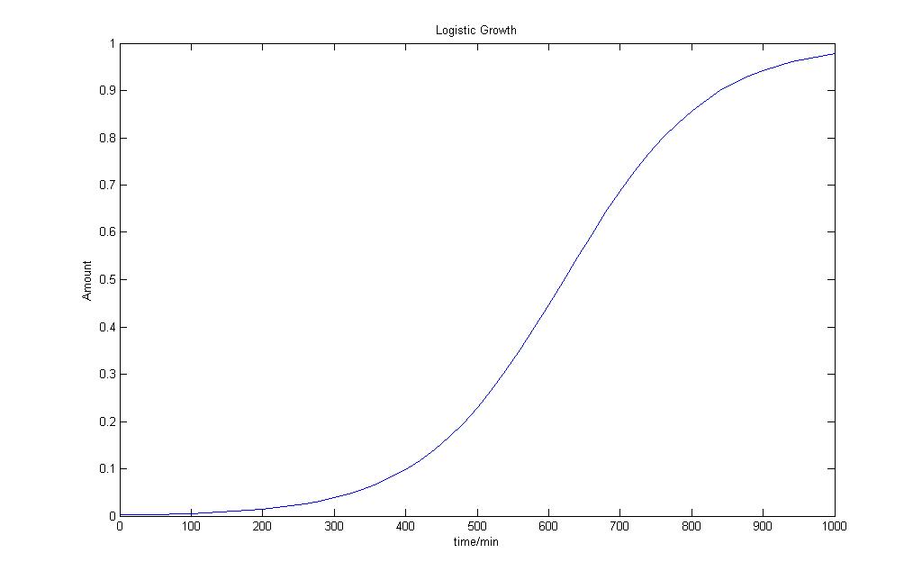
The logistic growth model is typically applied to growth kinetics of Microbes and other natural phenomena. This phenomena is based on the fact that no population can expand exponentially forever and there will be a certain limit to the number of species based on the space that is available.
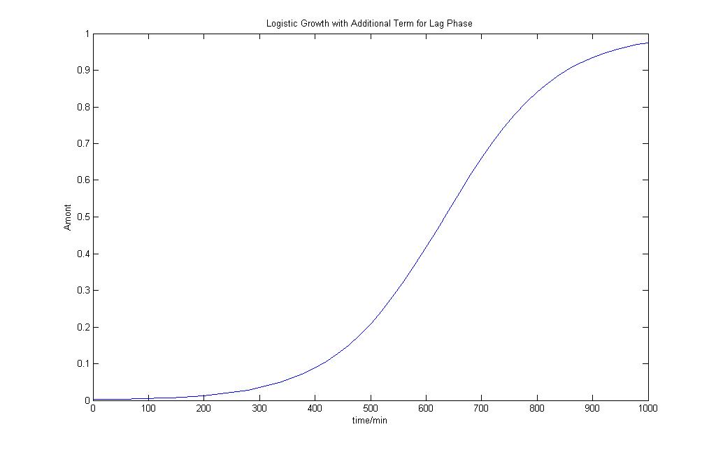
Here we explore the results of three Logistic Growth equations and their various outputs to see how well the results turn out to be.
Logistic Growth Model
| N = | number of species in the population |
| t = | time |
| Nmax = | Maximum number of species in the ecosystem |
| r = | intrinsic rate of natural increase |
Logistic Growth Model with lag phase
| Nmin = | Minimum number of species in the ecosystem |
| c = | Adjustment factor |
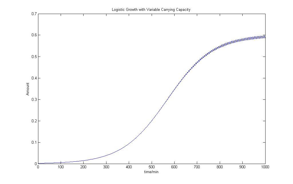
Logistic Growth Model with Varying Carrying Capacity
From the model, we can see that population that has an early exponential phase of growth and is not so affected by the variability in the carrying capacity. As the population reaches the limit, the population starts to oscillate at the same frequency as the carrying capacity and some of the population starts to die off.
We would use this as our logisitc equation model to add a bit more variability into our deterministic model.
Complex Formation
In an ODE model, a reaction network is expressed as a set of differential equations with one equation per chemical and with terms that represent the reactions. Our complex formation equation has ignored the fact that the reaction could be reversible. Here we add in a new complex formation equation to make our models more robust.
Using , and assuming mass action kinetics, the differential equation for C is
kf = forward reaction rate kr = reverse reaction rate
Links
Do refer to <span style="font-size:20pxParameter Estimation of GFP production system</span> for more details on the above parameters used.
Building the Construct
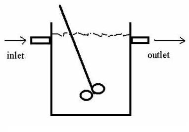
Revisiting the general idea of our modeling, we have treated each bacteria cell to work as a CSTR (Continuous stirred Reactor).
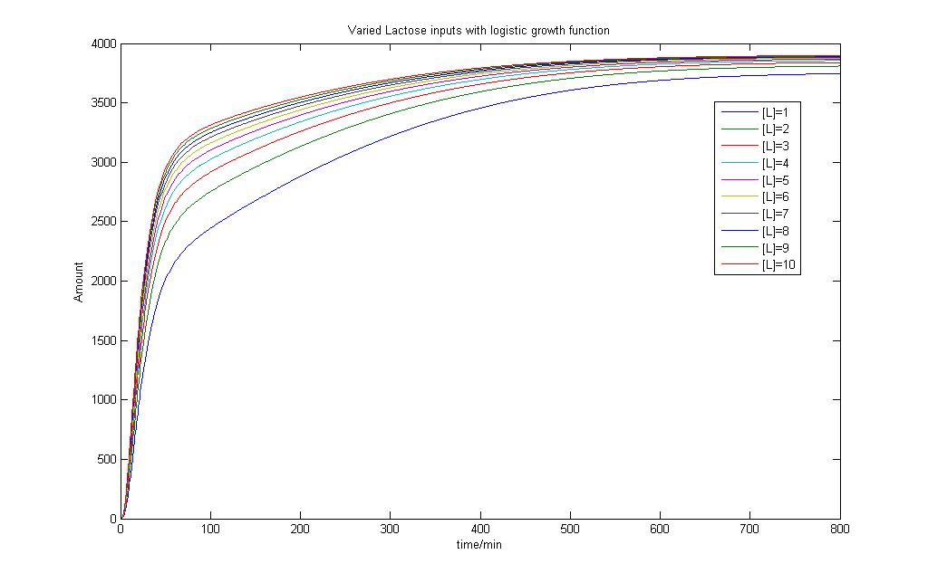
However, each bacteria is itself a reactor and these "mini reactors" multiply and grow~! Therefore we want our new model to be able to account for both the production of proteins and the growth pattern of the bacteria. So now instead of a simple basal signal into our model, we would send in a signal that codes for a "logistic growth" in the basal transcription of the model.
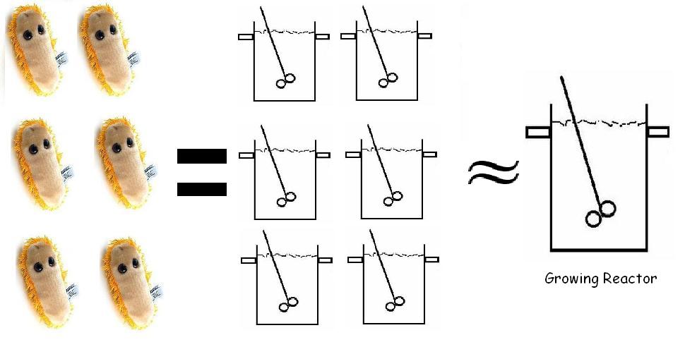
By giving our reactor model a signal to "grow", we can try to simulate this logistic growth output as observed in our experiments.
As seen, the logistic input can still capture varying lactose inputs and this model seems to be a more representative one for the characterization results. Interestingly, as lactose input increases, the model shows that the output changes less. We intend to use these results for our characterization experience and it will be found in the next section.
Correlation section
Correlations form an integral part in chemical engineering. Many phenomena observed in chemical processes have been extensively studied and relevant data collected to provide correlations between the variables of interest. This is to allow end users to be able to predict certain outcomes based on the knowledge of a specified variable if the correlation is availble. This practise is common when a process is not fully understood and a quick but efficient method to determine the process output is desired. Herein lies the aim of the next part of our project: to find a correlation between the amount of GFP produced and the fluorescence observed.
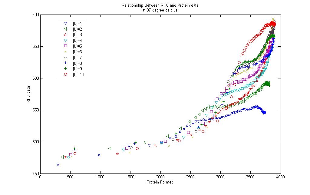
Model results and RFU data
A simple correlation was done between the model results and the RFU collected.
For the 10 graphs, correlations were generated for each of them using the [http://www.mathworks.com/products/curvefitting/ Curve Fitting toolbox] found in MATLAB.
The results are found in each of the links below. Each curve is shown together with the prediction bounds to a 95% cofidence level and the equation of the curve.
Lactose = 1mM
Lactose = 2mM
Lactose = 3mM
Lactose = 4mM
Lactose = 5mM
Lactose = 6mM
Lactose = 7mM
Lactose = 8mM
Lactose = 9mM
Lactose = 10mM
The curves were fitted once a R-square value of higer than 0.99 was obtained. Although the curves could be successfully obtained there remains some questions to be asked:
1) Is the model results truly representative of the real situation?
2) Will temperature changes have an impact on the results? However it is still possible that our model can account for temperature effects by tweaking the logistic growth input parameter. Recall that our model accounts for varying carrying capacity, and a different temperature could be represented by different paramter values.
References
1. A new logistic model for Escherichia coli growth at constant and dynamic temperatures FUJIKAWA Hiroshi ; KAI Akemi ; MOROZUMI Satoshi
 "
"


