Team:Imperial College/Growth Curve

From 2008.igem.org

Revision as of 04:00, 27 July 2009 by Chowes (Talk | contribs)
(diff) ← Older revision | Latest revision (diff) | Newer revision → (diff)


Modelling the Growth Curve

The first task of our dry lab team was to construct a simple yet effective model for the growth curve of B. subtilis. The inspiration for our model came from the work done by the Imperial College team on the characterisation of Cell Free Systems (here) and the elegant manner they found to couple the production terms in the model with the resources available in the medium.


The Model

Our model is based on the crucial role played by nutrients, and other resources, during the main growth phases that B. subtilis undergoes - the lag phase, the exponential phase and the stationary phase. To keep the model simple, we omit the fourth phase of growth - the death phase.

Lag phase.JPG
Lag Phase

During the lag phase, the rate of growth is slow. All nutrients are situated outside the cell initially. Some time is needed for an adequate amount of nutrients to move from the outside of the cell into the interior of the cell. This is vital, as the cell requires the nutrients for growth.

Exponential phase.JPG
Exponential Phase

Nutrients are consumed during cell growth and the growth is exponential as long as there are enough nutrients available. The exchange of nutrients ensures that the intra- and extracellular nutrient concentrations are the same.

Stationary phase2.JPG
Stationary Phase

The growth of the colony ceases in number and in volume. This happens when the colony has consumed all available nutrients. Other contributing factors may be death and cell division.

We chose to represent the growth in terms of overall volume rather than number of cells. For small volumes (lag phase and early exponential phase) the volume is a smoother variable (the overall volume grows a little in the lag phase) while in later phases, the volume and the number of cells are proportional.
Considering the overall volume also regularises the process since it allows us, to some extent, to overlook the process of cell division during the bacteria growth. We can assume the internal concentration of nutrients is reset almost instantaneously to the external concentration. During this time, the total volume does not change.

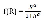
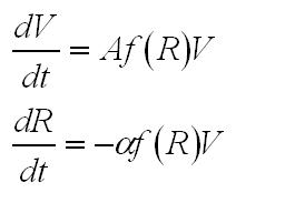
In order to couple growth with resources, our model curbs the optimal growth rate of the volume (A) as a function f of the resources R. We used a Hill function of exponent n, as it models with only one parameter the fact that production is unhindered when resources are plentiful and minimal when resources have run out. Finally we assume that in term of resources the cost of an extra unit of volume is alpha.

The growth of the overall volume V is therefore modelled as:
Growth equ.JPG

f(R) is the Hill function, where

Hill fn eq.jpg

Its switch point is 1.

The M-file we wrote for the growth model can be found in the Appendices section of the Dry Lab hub.


Results

As the simulation below shows, in a rich medium the nutrients are taken up quickly, resulting in a 'nutrient crash'. The transition from exponential to stationary phase is very sudden. In the case of our experimental data, the transition is much smoother and the growth far less explosive even in the exponential phase, thus suggesting that the growth medium was not very rich in nutrients and that even at the beginning of the exponential phase the growth was hampered.

Nutrient ft.JPGLabel model.JPG


The model for the growth curve was fitted to the experimental results. The results are shown below. The experimental results are depicted by the red curve, while our model is shown by the green curve. The resource curve was also plotted as a function of time and is shown below. It clearly confirms our initial guess regarding the poorness of the medium in term of nutrients.

It is worth noting that the model 'fit' is very good in the exponential and stationary phases. However, the fit is poorer in the lag phase. This suggests that the model should be expanded in order to take into account phenomena such as the movement of the nutrients into the cells.


Experimental Result.JPG
Fitted Curve.JPG
Resource Curve.JPG
Experimental Results
Fitted Curve
Resource Curve


The search for the optimal model parameters was done by brute force. But instead of browsing the whole space of parameters, we reduced the search volume with a simple pre-processing of the experimental data. The initial volume was estimated from the data - likewise the volume in the stationary phase which is directly related to the model parameters R0 and alpha. The model parameter A being related to the apparent growth rate of the experimental data, We plotted the log graph to determine the growth rate of our data.


Log-Graph used to determine the growth rate

Log-Graph used to determine the growth rate

The following constants were found to yield the best fit to experimental results:
- GROWTH CONSTANT (A): 1.3494
- INITIAL NUTRIENT CONCENTRATION (R0): 2
- HILL COEFFICIENT (n): 1.25
- INITIAL OD: 0.4
- CONSTANT (α): 0.64516