Team:UNIPV-Pavia/Modeling
From 2008.igem.org
Contents |
Mathematical modeling page
In this section we explain two dynamic models that can be used to describe the gene networks in our project. After a brief overview about the motivation of a mathematical model, we will illustrate the general formulas we used, we will show the complete ODE models for Mux and Demux gene networks, and then we will report results of some simulations performed with Matlab and Simulink.
Why writing a mathematical model?
The purposes of writing mathematical models for gene networks can be:
- Prediction: a good and well identificated model can be used in simulations to predict real system behavior. In particular we could be interested in system output in response to never seen inputs. In this way, the system can be tested 'in silico', without performing real experiments 'in vitro' or 'in vivo'.
- Parameter identification: we already wrote that it is very important to estimate all the parameters involved in the model, in order to perform realistic simulations. Another goal that can be reached with parameter identification is 'network summarization', in fact estimated parameters can be used as 'behavior indexes' for the network (or a part of it). These indexes can be very useful for synthetic biologists to choose and compare BioBrick standard parts for genetic circuits design, just like electronic engineers choose, for example, a Zener diode, knowing its Zener voltage.
Equations for gene networks
In this paragraph, mathematical modeling for gene and protein interactions will be described.
Binding of a ligand to a molecule: Hill equation
The fraction of a molecule saturated by a ligand ( = the probability that the molecule is bound to a ligand) can be expressed as a function of ligand concentration using Hill equation:
- Prob: the probability that the molecule is bound to the ligand
- [L]: concentration of the ligand
- K50: dissociation constant. It is the concentration producing a probability of 0.5
- n: Hill coefficient. It describes binding cooperativity
Regulated transcription
Transcription of a mRNA molecule can be regulated by transcription factors in active form. These factors can be activators or inhibitors: they respectively increase and decrease the probability that RNA polymerase binds the promoter. This probability must be function of active transcription factor concentration and can be modeled using Hill equation. If factor in active form activates transcription, we can write:
- Prob: probability that the gene is transcripted
- [T]: concentration of the transcription activator in active form
- K50: dissociation constant. It is the concentration producing a probability of 0.5
- n: Hill coefficient (n>0)
while, if factor in active form inhibits transcription, we are interested in unbound promoter and so we can write:
- Prob: probability that the gene is transcripted
- [T]: concentration of the transcription inhibitor in active form
- K50: dissociation constant. It is the concentration producing a probability of 0.5
- n: Hill coefficient (n>0)
The equations show that:
- In activation formula, if [T]=0 the trascription probability is Prob=0, while the maximum probability, Prob=1, is reached asymptotically for [T]->Inf
- In inhibition formula, if [T]=0 the trascription probability is Prob=1, while the minimum probability, Prob=0, is reached asymptotically for [T]->Inf
These formulas can be included in a differential equation that can describe the dynamic behavior of a mRNA molecule as a function of the factor that regulates its transcription.
ODE for activated transcription
- Vmax: maximum transcription rate
- [m]: concentration of mRNA molecule
- [T]: concentration of the transcription activator in active form
- K50: dissociation constant
- n: Hill coefficient (n>0)
- delta: mRNA degradation constant
- a: leakage factor that can modellize promoter basic activity. It is a percentage of Vmax
ODE for inhibited transcription
- Vmax: maximum transcription rate
- [m]: concentration of mRNA molecule
- [T]: concentration of the transcription inhibitor in active form
- K50: dissociation constant
- n: Hill coefficient (n>0)
- delta: mRNA degradation rate
- a: leakage factor that can modellize promoter basic activity. It is a percentage of Vmax
ODE for constitutive transcription
- c: constant transcription rate
- [m]: concentration of mRNA molecule
- delta: mRNA degradation rate
Transcription factors in active form
Formulas described so far are dependent on the concentration of transcription factor in active form. But how can we calculate the amount of transcription factor in active form? Assuming that the transcription factor can be activated or inhibited by a inducer factor (that can be an exogenous input), we can use Hill equation again to calculate the concentration of bound and unbound transcription factor as a function of the inducer factor:
- [I]: concentration of the inducer
- [T]t: total concentration of the transcription factor
- [T]u: concentration of unbound transcription factor
- [T]b: concentration of bound transcription factor
- K50: dissociation constant
- n: Hill coefficient (n>0)
If active form is bound transcripion factor, we are interested in Tb, while if active form is unbound transcription factor, we are interested in Tu.
ODE for protein production
We have to modellize translation of mRNA molecules. We chose to describe it as a differential equation in which protein production and protein degradation are linear:
- [P]: concentration of protein
- [m]: concentration of mRNA molecule
- alpha: translation rate
- beta protein degradation rate
Our model
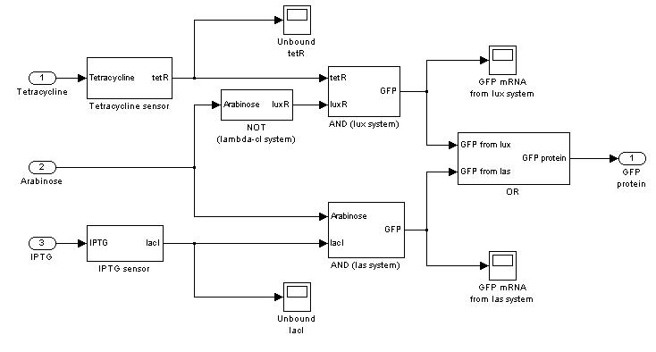
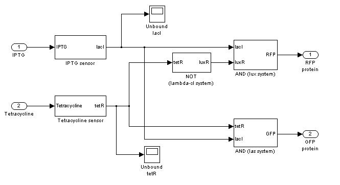
We considered Tetracycline, IPTG, Arabinose and GFP respectively as CH0, CH1, SEL and OUT signals for Mux, while we considered IPTG, Tetracycline, RFP and GFP respectively as IN, SEL, OUT0 and OUT1 signals for Demux. For all these signals, logic 1 corresponds to the presence of the molecule.
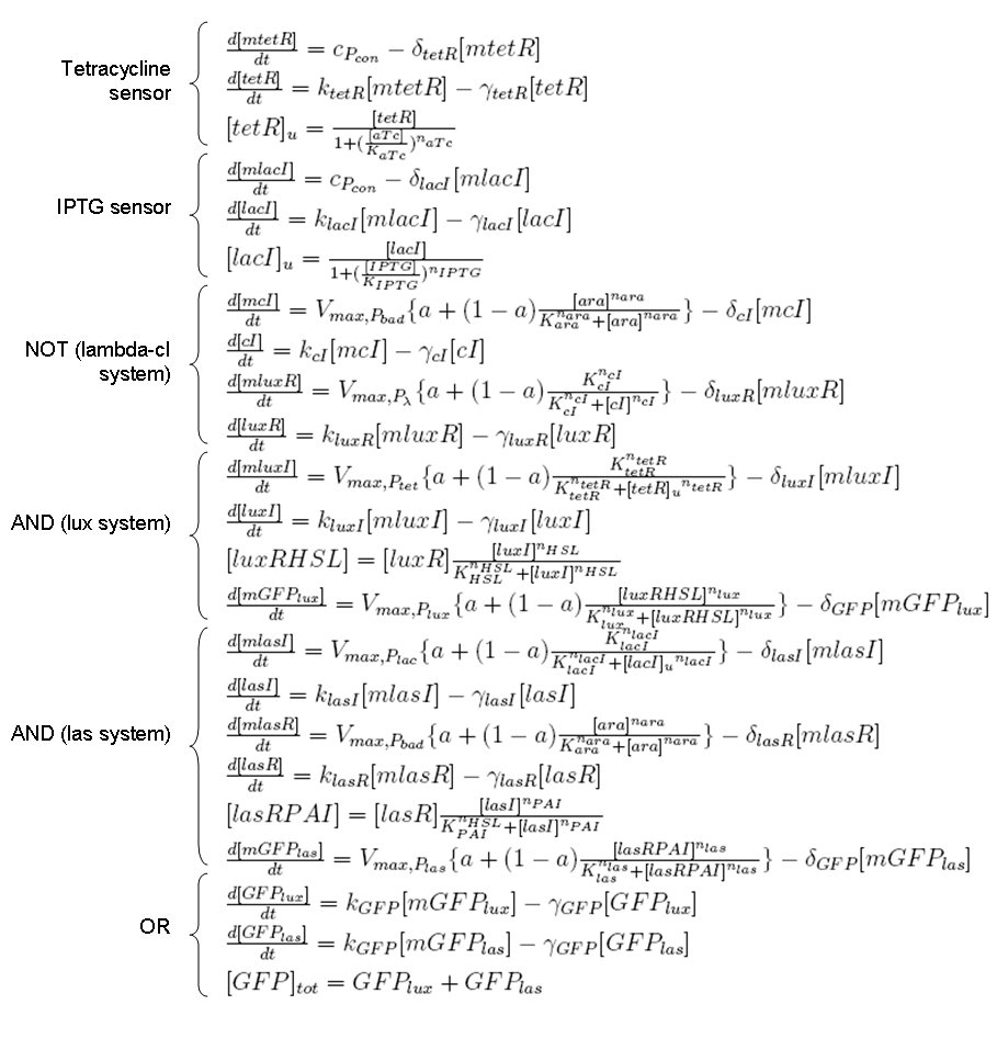
According to the equations described so far, every protein and mRNA is a state variable for the model. Mux and Demux models are described in the next paragraphs.
We considered full ODE models, in which transcription and translation processes are separated. In many contexts, anyway, we can write only one differential equation to describe a "regulated protein production", in which trascription process is hidden. In this section we preferred to be general and we considered the transcription dynamic because our aim is to provide a mathematical model for future parameter identification. We also decided to neglect AHL synthesis dynamic, considering luxI protein a "direct" activator for luxR.
In the following paragraphs, the complete ODE systems and the Simulink block diagrams will be reported.
Mux
Demux
Simulations
The written models have been simulated in Matlab and Simulink, in order to perform a preliminary heuristic study of the system behavior and to search for critical parameters. For simulations, we used dimensionless ODEs to avoid numeric errors due to small parameter values, so results are reported in arbitrary units. We defined ODE systems in Simulink (block diagrams showed above) and then solved them using ode15s, a multistep ODE solver for stiff problems.
Parameters have been calibrated considering the values reported in literature and in some other iGEM wiki pages. In some cases values were missing, so we fixed these missing values at 1*10^om, where "om" is the median order of magnitude of the parameters having the same meaning (e.g. protein degradation rates).
In other cases we found different values for the same parameter, so we computed the mean value.
An important feature that will have to be studied is systems' basic activity. In other words, can genetic Mux discriminate the output in response to a low input signal and the output in response to a high input signal? Moreover, does Demux have a non negligible baseline activity that turns on the output channel that should be unactive? One of the parameters that plays a very important role in basic activities is the leakage factor ("a", that is the probability that a mRNA is transcribed randomly). This parameter depends on the specific promoter. Future estimation of "a" for all the promoters will be useful to predict "false positive" system outputs. High "a" values give high basic activities, while for a->0 transcriptional regulation becomes "ideal".
At first, we wrote the ODE models with only one "a" parameter, but then we decided to consider different leakage factors for the promoters in the network.
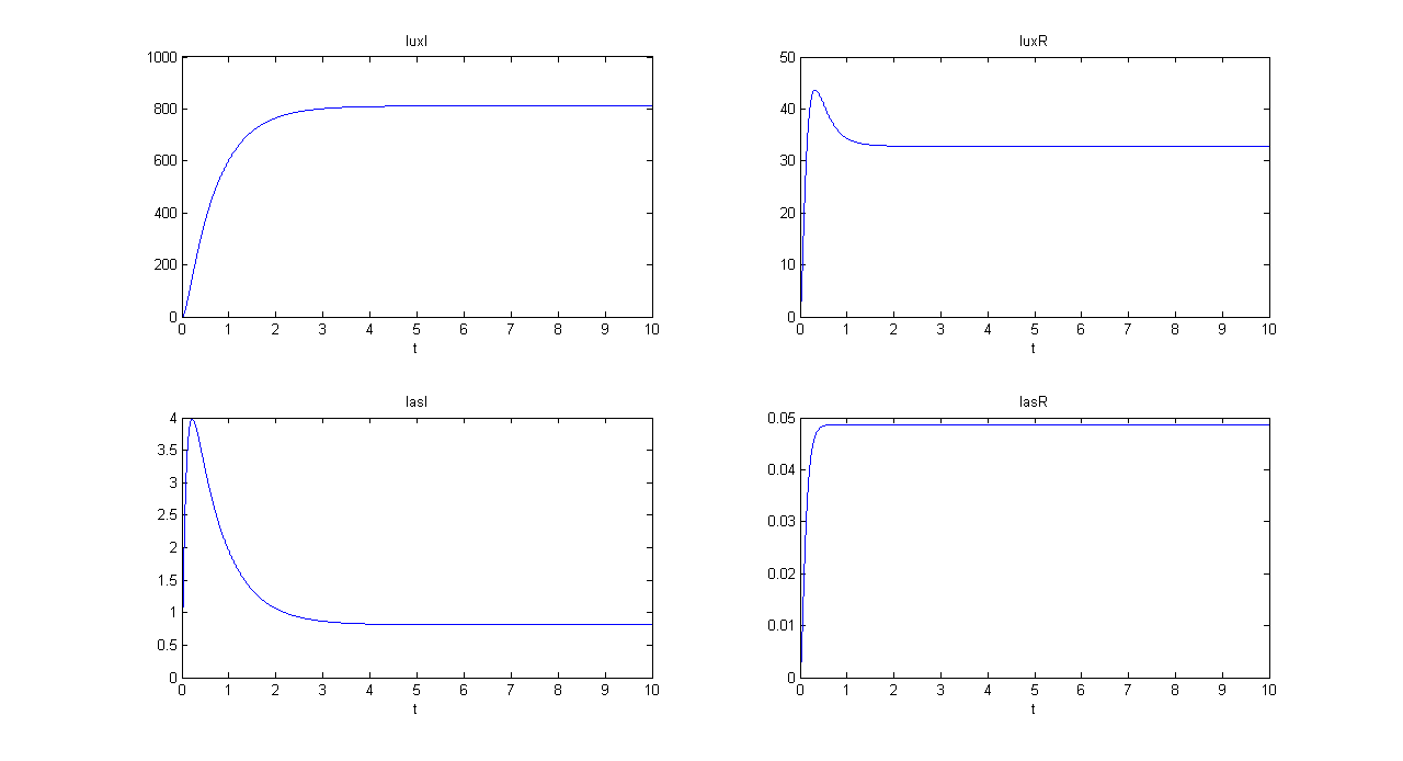
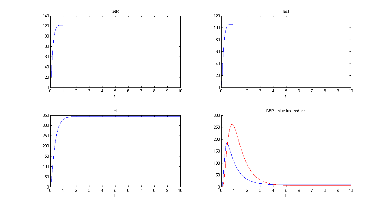
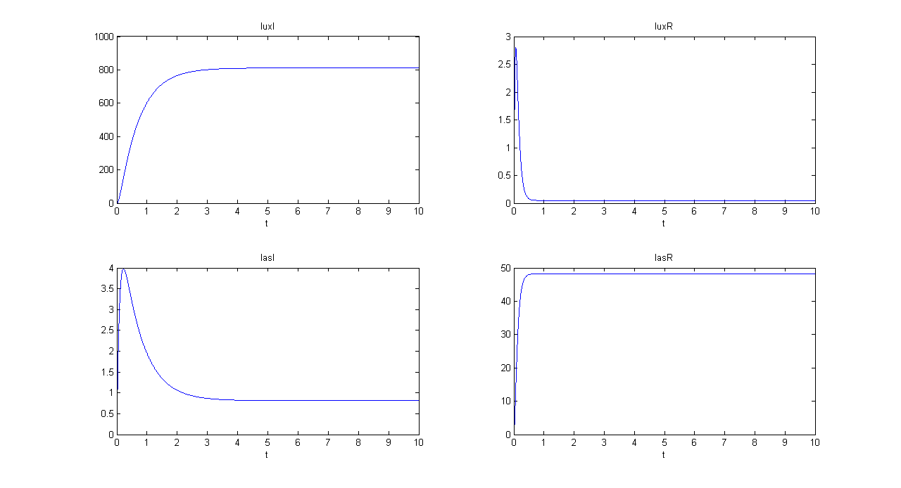
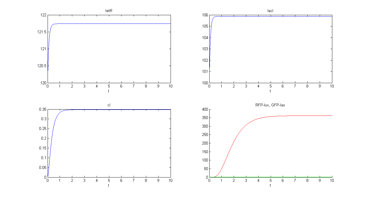
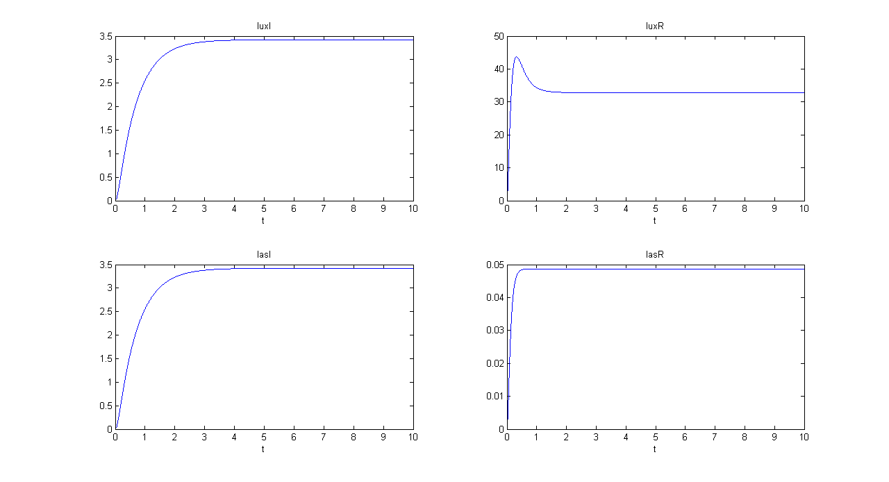
Here we report some simulation examples. The initial states (t=0) have been fixed to 0, but here we are interested into steady state values.
Mux
We distinguished lux and las system contributions for output GFP.
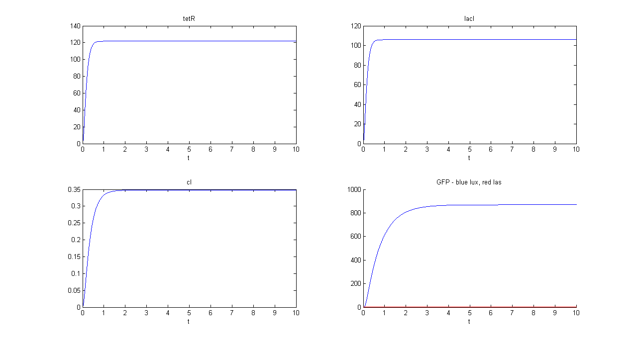
SIMULATION 1
- Tetracycline = 10
- IPTG = 0
- Arabinose = 0
- Tetracycline channel (CH0) is selected and Tetracycline is present, so we expect to find a high GFP(lux) value and a low GFP(las) value.
- Comments: GFP(las) in low, but not null, because of leakage factor. Posing "a"=0, GFP(las) becomes null. Mux output is the sum of GFP(lux) and GFP(las). If we sum these values at steady state, we have 870.2330 (arbitrary units).
SIMULATION 2
- Tetracycline = 10
- IPTG = 0
- Arabinose = 10
- IPTG channel (CH1) is selected, but IPTG is not present, so we expect to find low steady state GFP values for both lux and las systems.
- Comments: total GFP is low after a transient time. If we sum GFP(lux) and GFP(las) values, we have 14.2292 (arbitrary units), that is much lower than the output total value in SIMULATION 1, confirming that the chosen parameter set gives low leakage.
Demux
SIMULATION 1
- Tetracycline = 0
- IPTG = 0
- IPTG signal (INPUT) is absent, so we expect to find a low RFP and GFP values.
- Comments: RFP and GFP values are not null, because of leakage. The numeric steady state values are 0.869 for GFP and 2.8753 for RFP, in arbitrary units.
SIMULATION 2
- Tetracycline = 0
- IPTG = 10
- IPTG signal (INPUT) is present and Tetracycline signal is not. So, INPUT is transferred into RFP channel (OUT1).
- Comments: GFP steady state value (0.8709 arbitrary units) is comparable to GFP value in SIMULATION 1. This value is much lower that RFP steady state value (362.11 arbitrary units), confirming that the selected output channel have a significantly higher output value.
All these simulations will have to be supported with experimental results and parameters will have to be identified in order to characterize our physical devices.
References
[1] Modelli multiscala per studi di proteomica e genomica funzionale, S. Cavalcanti, S. Furini, E. Giordano. "Genomica e proteomica computazionale", GNB Book, Publisher: Pàtron, 2007
[2] ETH Zurich iGEM 2007 Wiki - Modeling basics page
 "
"


