|
_modeling
Introduction
Dimerization of the extracellular receptor domains is an important necessity for the functionality of our Modular Synthetic Receptor System. Presenting the system a stimulus in the form of spatial arranged ligands results in dimerization of the extracellular domains and thus the corresponding intracellular parts such as the split lactamase halves or split fluorescent proteins complement to a measurable output. To analyze the functionality due to dimerization, first two receptor dimerization models (one T cell receptor model and one general receptor model) are introduced and discussed and then a proper model for the Modular Synthetic Receptor System is constructed.
As given by the diversity of our transmembrane fusion proteins, some of the constructs can bind fluorescein as ligand as well. As the model for the Modular Synthetic Receptor System is applicable for all our constructs, the ligand usage is extended with fluorescein. So either NIP or fluorescein can function as ligand, dependent on the choice of constructs for implementation.
T cell receptor dimerization model I
matlab m-file
T cells are a special type of white blood cells (lymphocytes) and play a central role in cell-mediated immunity. They carry special receptors, so called T cell receptors (TCR) on their membrane. One part of the mechanisms to activate a TCR and thus to activate a T cell is the binding of a ligand, also called antigen, to the TCR. As research showed, one single ligand-TCR complex does not lead to a T cell response yet, as at least two ligand-TCR complexes and their dimerization seem to be required for proper T cell activation (Schamel, 2006; Bachmann 1999).
In our case the ligands are nitro-iodo-phenol (NIP) molecules attached to a DNA-Origami structure at a (variable) distance of ~6nm to each other. These NIPs are recognized and bound by the TCRs. As the distance is small enough for two TCRs to approach very closely when each of them binds a NIP, they can dimerize.
A simplified pathway shows the extracellular sequence of TCR activation. After the NIP binding two complexes come together and form a dimer which then leads to activation of the TCR and further intracellular signaling and T cell activation.
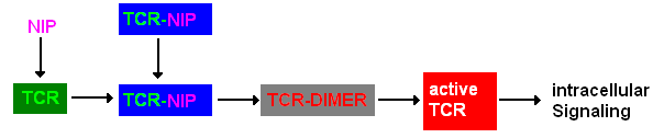 Figure 1: Pathway of TCR dimerization |
Reaction kinetics
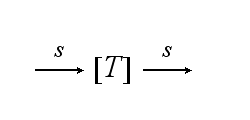
The T cell maintains a pool of TCRs (T) which is dynamic. The continuous de novo expression, random internalization and degradation runs with constant rate S :
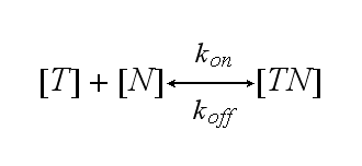
One NIP molecule (N) binds to a TCR (T) with the reaction rate kon or a TCR-NIP complex (TN) dissociates with the reaction rate koff :
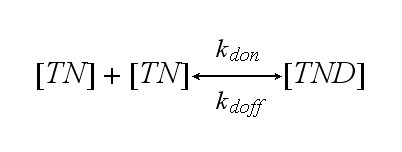
Two TCR-NIP (TN) complexes dimerize to a TCR-NIP dimer (TND) with rate kdon ; the dissociation of a TCR-NIP dimer runs with rate kdoff :
In order to get active TCRs, the TCR-NIP dimer (TND) has to switch into two active TCRs (A) with rate ka :
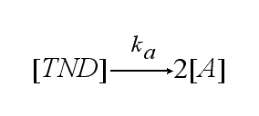
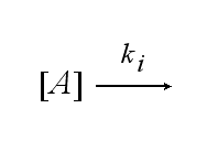
After activation, the TCR is internalized with rate ki and does not take part anymore in the extracellular signaling :
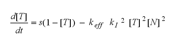
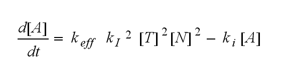
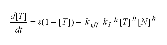
ODEs derived from the kinetics (Details)
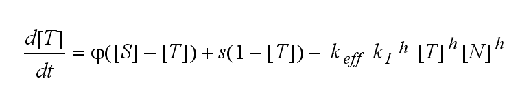
In the following equation T represents the free TCR in the T cell membrane where keff is a combination of kdon, kdoff and ka. kI is kon/koff :
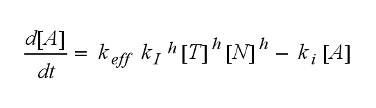
The equation for the active TCR A is shown in the following:
TCR activity for a set of parameters
The two ODEs above of this first basic model for a set of parameters are solved numerically. They reveal the time course of the TCR activity and the time course of the unbound TCR aswell.
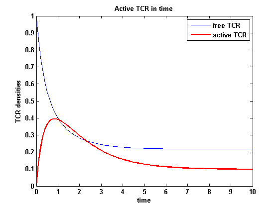 Figure 2: TCR densities in time |
chosen parameters:
s = 0.1;      % turnover rate
kon = 1;      % TCR-NIP binding rate
koff = 0.2;   % TCR-NIP dissociating rate
kdon = 1;     % TCR-NIP dimerization rate
kdoff = 0.2;  % dimer dissociating rate
ka = 1;       % activation rate
ki = 0.8;     % internalization rate
N = 0.2;      % NIP amount
initial integration conditions:
T0 = 1    % free TCR density
TA0 = 0;  % active TCR density
|
The activity has a maximum a short time after NIP presentation and decreases as the active TCRs are internalized and as the free membrane TCR amount is decreasing. It is remarkable that the response never decreases to complete zero, even for very high internalization rates and in a long time course.
Extensions: Ultrasensitivity and biphasic kinetics
matlab m-file
Ultrasensitivity
The kinetics of the TCR activation can be generalised by substituting the second order kinetic of the ligand N and the receptor T by a parameter h, which then represents the kinetic order of the system.
Now the sensitivity of the model to ligand and receptor is altered aswell. It increases when the kinetic order increases. For a high kinetic order, small changes in ligand N or receptor T cause big changes in the TCR activation (A). Generally h can be described as:
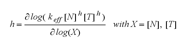
This logarithmic sensitivity means that the increasing of the concentration of N with 10% will lead to an increase in the rate of TCR activation of 10000% for the 4th order kinetic (h=4).
Not all TCRs on a T cell membrane can be recruited to NIP binding as a cell´s membrane contains several transmembrane proteins whose size can avoid a TCR-NIP formation when they surround a TCR and make the approaching of the NIP to the binding side of the TCR impossible. Considerating this spatial barriers leads to the idea of a TCR which can switch between two states, one binding state and one non-binding state. Hence a introduction of two different pools of TCRs into the model is appropriate. If a TCR is not available for a NIP molecule, thus it is in the non-binding state, it belongs to the so called spare pool, whereby TCRs belonging to the so called interface pool are in the binding state and can be accessed by the NIP molecule. Moreover the spare pool is in dynamical exchange with the interface pool, so non-binding TCRs can become binding TCRs. This exchange is regulated through the parameter λ, a ratio between the spare and the interface pool and φ, the exchange rate constant. S is the spare pool TCR density and T the TCR density of the interface pool. A represents the active TCR density. So the full model I equations are:
Spare pool:
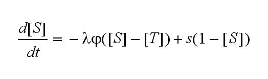
Interface pool:
Active TCR:

TCR activity dependent on exchange rate φ and ratio λ :
(Extract from parameter analysis)
The dependency of the activity on λ and φ is shown in the following:
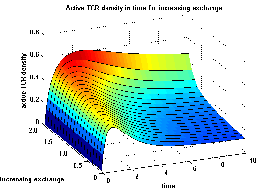 Figure 3: Active TCR density in time for different exchanges |
chosen parameters:
s = 0.1;      % turnover rate
kon = 1;      % TCR-NIP binding rate
koff = 0.2;   % TCR-NIP dissociating rate
kdon = 1;     % TCR-NIP dimerization rate
kdoff = 0.2;  % dimer dissociating rate
ka = 1;       % activation rate
ki = 1;       % internalization rate
N = 0.2;      % NIP amount
h = 2;        % kinetic order
initial integration conditions:
S0 = 1;    % spare TCR density
T0 = 1;    % interface TCR density
TA0 = 0;   % active TCR density
|
The x-axis represents the time course of the activity, the y-axis represents both parameters φ ( = y) and λ ( = 2 - y). So each black line in the plot is a time course of the TCR activity for a different φ and λ. The z-axis is the response intensity. With increasing exchange between the interface and spare pool, more TCRs switch to the binding state, hence more TCRs can bind NIP. As a consequence the active TCR density is higher than for a low exchange.
Correction terms
matlab m-file
Regarding the reaction kinetics and considering the ODEs as a model for TCR dimerization (Bachmann, 1999) led to the realization of an error in the mentioned publication. The ODEs evolved from the reaction kinetics are not :
but :
Furthermore can be derived for the NIP density and the free TCR:
The NIP density is not a static value anymore but time dependent also.
On that account the last five equations are the corrected model equations. Solving this five equations numerically for a set of parameters gives a similar time course of the active TCR density but the response strength is lower than in the original version, although the initial NIP amount is five times higher:
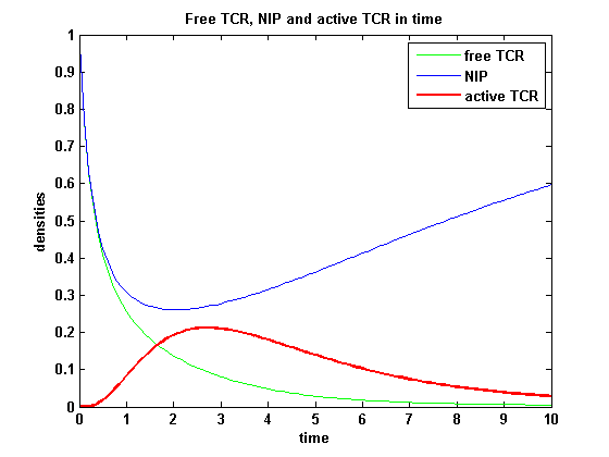 Figure 4: Time course of NIP, free TCR and active TCR for a set of parameters |
chosen parameters:
s = 0.1;      % turnover rate
kon = 3;      % TCR-NIP binding rate
koff = 0.1;   % TCR-NIP dissociating rate
kdon = 1;     % TCR-NIP dimerization rate
kdoff = 0.2;  % dimer dissociating rate
ka = 1;       % activation rate
ki = 0.8;     % internalization rate
initial integration conditions:
N0 = 1;    % NIP amount
T0 = 1     % free TCR density
TN0 = 0    % TCR-NIP monomer density
TND0 = 0   % TCR-NIP dimer density
TA0 = 0;   % active TCR density
|
After NIP addition the TCR activity rises to a maximum and decreases as active receptors are internalized and the NIP amount is used up. The free receptor density recovers due to permanent expression of new receptors which are built into the membrane.
Receptor dimerization model II
matlab m-file
A receptor dimerization can proceed in a different way aswell, especially when two ligand molecules are linked to a structure like our DNA-Origami:
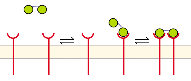 Figure 5: Pathway of receptor dimerization due to bivalent ligand |
Before the first step the receptors are unbound and diffuse in the cell´s membrane. The DNA-Origami binds to a receptor in the way that only one NIP molecule is connecting to one receptor. In the second step the second NIP molecule binds to the second receptor and both receptors dimerize.
Reaction kinetics
The continuous production of the cell´s receptor R with rate s is:
One receptor R binds to one of two NIP molecules NN of the DNA-Origami with rate kon or a receptor-NIP complex RNN dissociates with koff:
The second receptor R binds to the second NIP molecule of the DNA-Origami and both receptors dimerize with rate kdon or the dimer RNNR dissociates in one receptor R and one receptor-NIP complex RNN with rate kdoff:
The two receptors get activated with rate ka:
After activation the receptor is internalized with the ki:
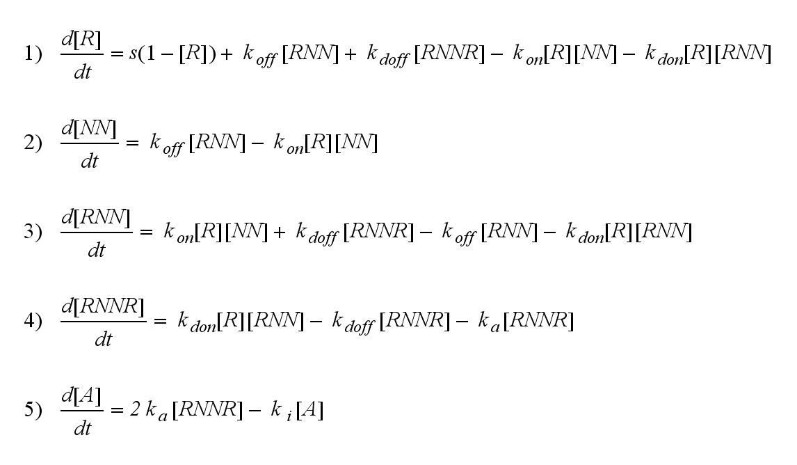
ODE derivation
The ODEs are derived from the reaction kinetics:
For a set of parameters the ODEs are solved and reveal amongst the other quantities the receptor densities in the time course:
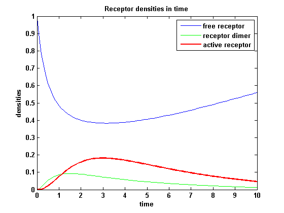 Figure 6: Receptor densities in time (model 2) |
chosen parameters:
s = 0.1;      %turnover rate
Kon = 3;      %binding rate
Koff = 0.1;   %dissociating rate
Kdon = 1;     %dimerization rate
Kdoff = 0.2;  %dimer dissociating rate
Ka = 1;       %activation rate
Ki = 0.8;     %internalisation rate
initial integration conditions:
R0 = 1;      %receptor density
NN0 = 0.5;   %NIP Amount
RNN0 = 0;    %receptor-NIP monomer
RNNR0 = 0;   %receptor-NIP dimer
A0 = 0;      %active receptor
|
The receptor activity rises after NIP addition, has a maximum and decreases due to the internalization of the active receptor. The dimer density increases fast after addition of NIP and decreases as dimers fade into active receptors.
Discussion of model I and II
For comparison, the ODEs of the corrected model 1 and model 2 are taken.
The receptor NIP binding mechanism differs in the two models. Model I assumes the production of two independent receptor-NIP complexes which can dimerize after formation. In model II, dimerization happens after one of two receptors connects to the bivalent ligand . Setting several conditions unravels the consequences of this differences for the active receptor, the dimer and the receptor recovery. Different binding rates, dimerization rates and ligand amounts are used in the solutions of the model I ODEs and model II ODEs.
Receptor densities dependent on binding rate kon
The two model ODEs are solved for the mentioned parameters below whereby the binding rate kon was variated.
So the course in time for the free receptor, the monomeric receptor-NIP complex, the dimer and the active receptor is plotted:
|
chosen parameters:
s = 0.1;        % turnover rate
kon : variated  % receptor-NIP binding rate
koff = 0.1;     % receptor-NIP dissociating rate
kdon = 1;       % receptor-NIP dimerization rate
kdoff = 0.2;    % dimer dissociating rate
ka = 1;         % activation rate
ki = 0.1;       % internalization rate
initial integration conditions:
free receptor : 1;
receptor-NIP monomer, dimer : 0;
Ligand/NIP density:
 Model 1: 0.5;
 Model 2: 0.25;
 As the ligand in model 2 is bivalent, the amount
 of initial NIP molecules is equal in both models.
|
kon = 0.2 :
| Model I | Model II |
|---|
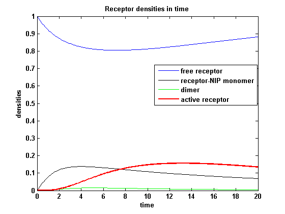 Figure 7.1: Receptor densities according to model 1 for binding rate = 0.2 |
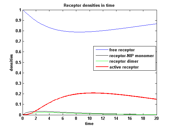 Figure 7.2: Receptor densities according to model 2 for binding rate = 0.2 |
kon = 3 :
| Model I | Model II |
|---|
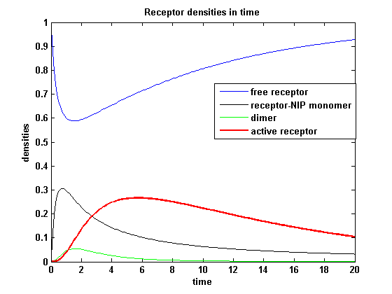 Figure 8.1: Receptor densities according to model 1 for binding rate = 3 |
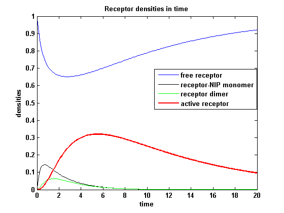 Figure 8.2: Receptor densities according to model 2 for binding rate = 3 |
receptor activity for different kon :
| Model I | Model II |
|---|
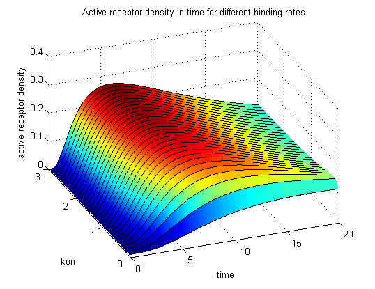 Figure 9.1: Receptor activity according to model 1 for different binding rates |
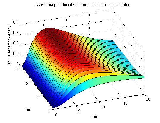 Figure 9.2: Receptor activity according to model 2 for different binding rates |
The production of receptor-NIP complexes is lower in model 2 than in model 1. Increasing kon leads to an increase in the formation of receptor NIP-complexes thus to a higher dimerization and receptor activation in both models. In model 1 receptor-NIP densities have approximately the same maxima as the active receptor densities and in model 2, receptor-NIP densities are much lower than active receptor densities. Active receptor densities react in both models similar to kon variations for the used parameters.
Receptor densities dependent on dimerization rate kdon
Applying different kdon leads to the following result:
|
chosen parameters:
s = 0.1;        % turnover rate
kon = 3;        % receptor-NIP binding rate
koff = 0.1;     % receptor-NIP dissociating rate
kdon : variated % dimerization rate
kdoff = 0.2;    % dimer dissociating rate
ka = 1;         % activation rate
ki = 0.1;       % internalization rate
initial integration conditions:
free receptor : 1;
receptor-NIP monomer, dimer : 0;
Ligand/NIP density:
 Model 1: 0.5;
 Model 2: 0.25;
 As the ligand in model 2 is bivalent, the amount
 of initial NIP molecules is equal in both models.
|
kdon = 0.3 :
| Model I | Model II |
|---|
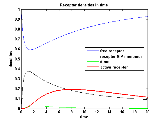 Figure 10.1: Receptor densities according to model 1 for dimerization rate = 0.3 |
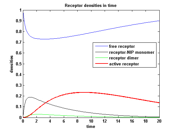 Figure 10.2: Receptor densities according to model 2 for dimerization rate = 0.3 |
kdon = 3 :
| Model I | Model II |
|---|
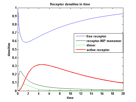 Figure 11.1: Receptor densities according to model 1 for dimerization rate = 3 |
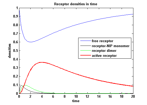 Figure 11.2: Receptor densities according to model 2 for dimerization rate = 3 |
receptor activity for different kdon :
| Model I | Model II |
|---|
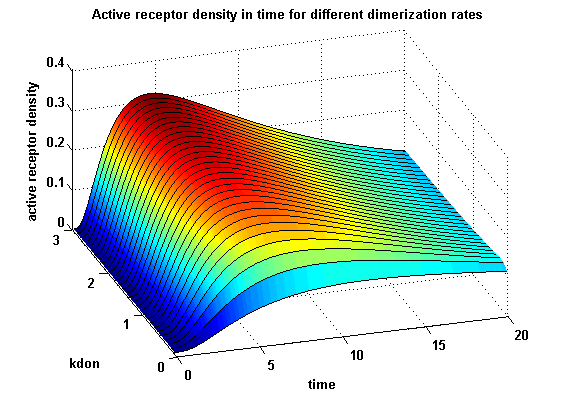 Figure 12.1: Receptor activity according to model 1 for different dimerization rates |
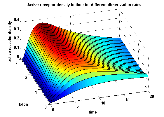 Figure 12.2: Receptor activity according to model 2 for different dimerization rates |
A low kdon gives in both models a high receptor-NIP monomer density as few of this complexes are recruited to build dimers and remain receptor-NIP monomers. This density decreases for high kdon due to a higher dimerization and receptor activity. kdon variations give similar changes in receptor activity in both models.
Receptor densities dependent on NIP amount
The use of different amounts of ligand is maybe the most important influence on the receptor activation. As the ligand is the stimulus in order to activate our system, it´s amount will determine strongly the activity of the receptor. So different amounts of NIP are used and a higher internalization rate ki is used aswell.
|
chosen parameters:
s = 0.1;        % turnover rate
kon : 3         % receptor-NIP binding rate
koff = 0.1;     % receptor-NIP dissociating rate
kdon = 1;       % receptor-NIP dimerization rate
kdoff = 0.2;    % dimer dissociating rate
ka = 1;         % activation rate
ki = 0.8;       % internalization rate
initial integration conditions:
free receptor : 1;
receptor-NIP monomer, dimer : 0;
Ligand/NIP density:
 Model 1: variated;
 Model 2: variated;
 Variating in a way that the parameter in model 1 is always
 double as high as the parameter in model 2 gives equal amounts of
 NIP molecules as stimulus, because the ligand in model 2 is bivalent
|
NIP = 0.1 :
| Model I | Model II |
|---|
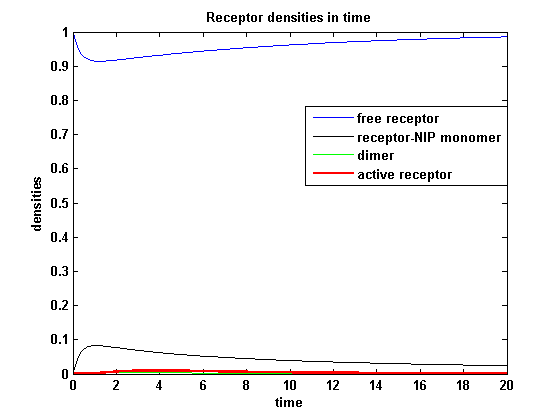 Figure 13.1: Receptor activity according to model 1 for a low amount of NIP |
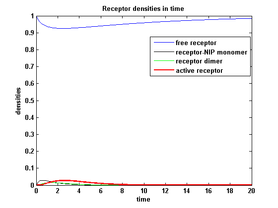 Figure 13.2: Receptor activity according to model 2 for a low amount of NIP |
NIP = 3:
| Model I | Model II |
|---|
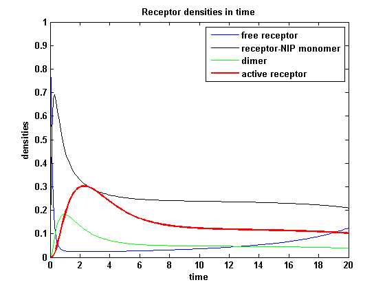 Figure 14.1: Receptor activity according to model 1 for a high amount of NIP |
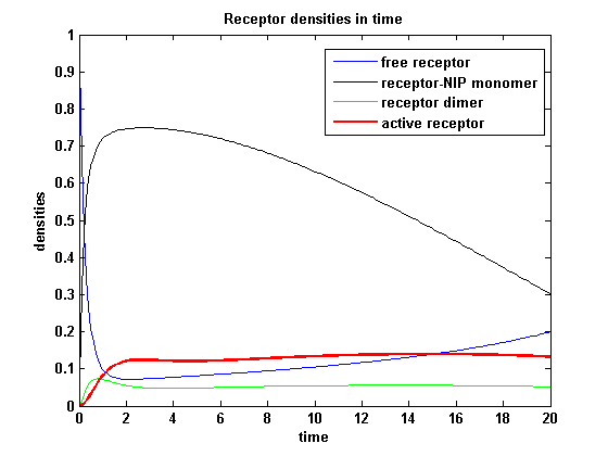 Figure 14.2: Receptor activity according to model 2 for a high amount of NIP |
receptor activity for different amounts of NIP:
| Model I | Model II |
|---|
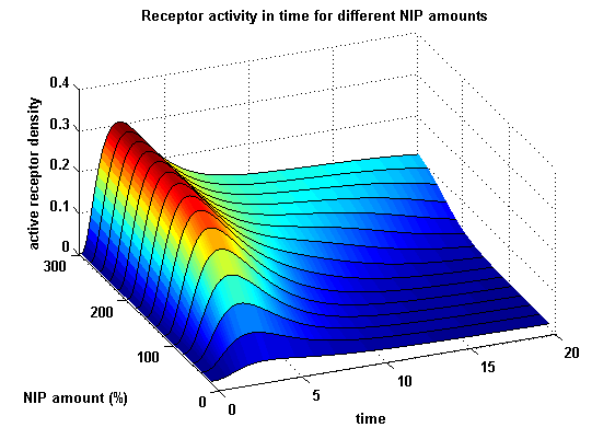 Figure 15.1: Receptor activity according to model 1 for different amounts of NIP (shown in % of initial free receptor amount) |
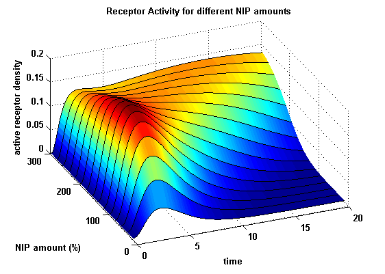 Figure 15.2: Receptor activity according to model 2 for different amounts of NIP (shown in % of initial free receptor amount) |
As ki=0.8, the receptor activity is decreasing due to a fast internalization of active receptors. For a little stimulus the active receptor activity is almost zero. Increasing the amount of NIP leads in both models to an increase of the active receptor density. It saturates for increasing amounts of NIP in model 1. In model 2 the active receptor density increases for increasing NIP amounts, but when the NIP amount reaches a certain level, it starts to decrease as too much receptor-NIP complexes are formed, leaving few receptors for dimerization. Aswell there can be observed a late activation for high NIP amounts in model 2.
Modular Synthetic Receptor System model
matlab m-file
The dimerization model II is used to form the base of the model for our Modular Synthetic Receptor System. It has two receptors R1 and R2. The bivalent ligand are two NIP molecules NN which are linked to DNA-Origami. Aswell two linked fluorescein molecules, or one NIP and fluorescein can serve as the bivalent ligand. Each receptor consists of a extracellular detector domain, which is connected to an intracellular split protein half by a short transmembrane protein. Only when receptor R1 and R2 dimerize, the intracellular split protein halves complement to become the complete functional protein A in the form of a β-lactamase or a fluorescent protein. A dimerization of R1 and R1 or R2 and R2 can happen to R1R1 or R2R2, but does not lead to an active intracellular protein and measurable output. Of course all receptor dimers (R1R2, R1R1, R2R2) dissociate into monomers much easier than a receptor dimer which is active in the form of A, as the connected split protein halves are bound to each other.
Reaction kinetics
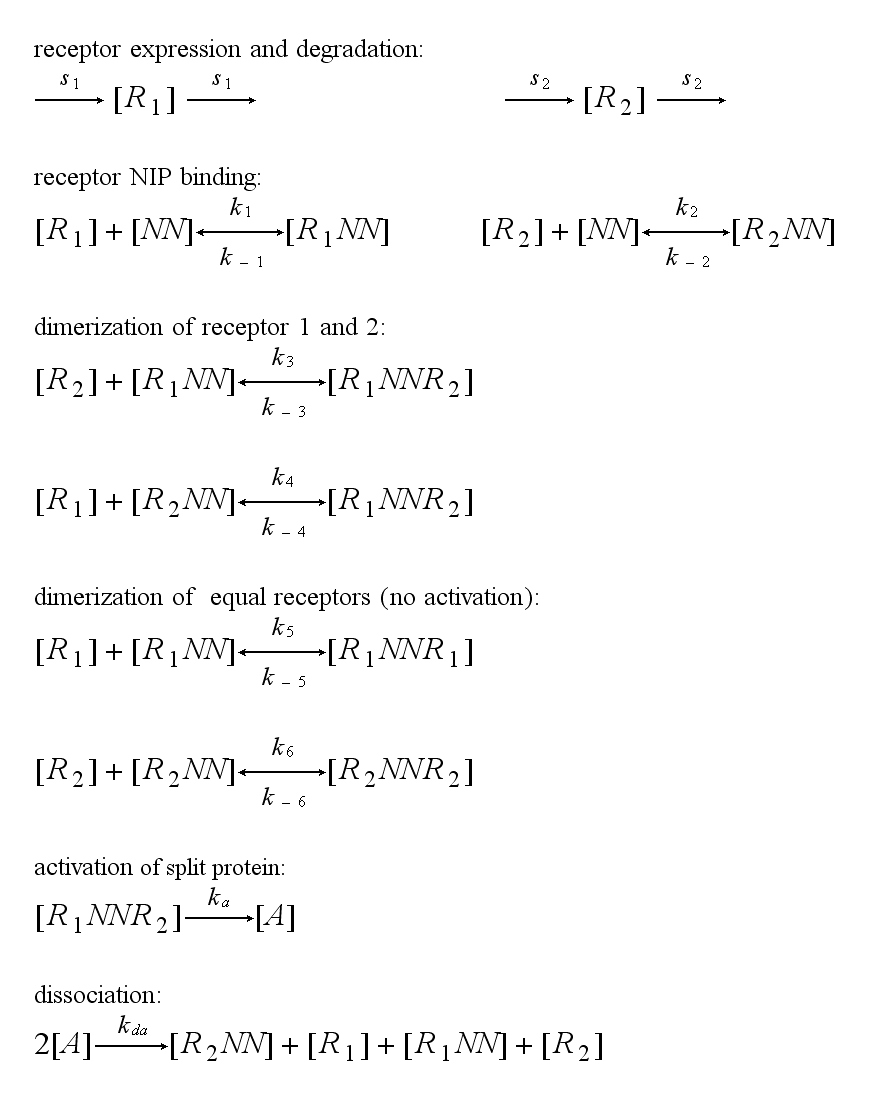
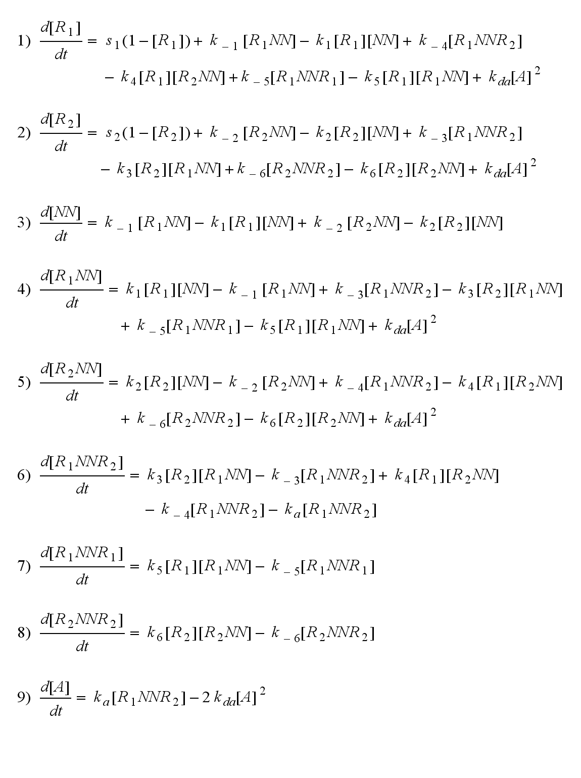
ODE derivation
The ODEs can be derived from the reaction kinetics again and are:
Involved quantities and split protein activity
The ODEs are solved for a set of parameters and reveal the time courses of the quantities:
 Figure 16: Involved receptor densities in time Assuming equal parameters for R1 and R2 leads to equal densities of both; shown through one plot curve for each uniform density (free receptor density, monomeric density, dimeric density) of R1 and R2
|
chosen parameters:
s1 = 0.1;   %turnover rate for R1
s2 = 0.1;   %turnover rate for R2
K1 = 3;     %binding rate 1
k1 = 0.1;   %dissociating rate 1
K2 = 3;     %binding rate 2
k2 = 0.1;   %dissociating rate 2
K3 = 2;     %R1R2 dimerization rate 1
k3 = 0.1;   %R1R2 dimer dissociating rate 1
K4 = 2;     %R1R2 dimerization rate 2
k4 = 0.1;   %R1R2 dimer dissociating rate 2
K5 = 2;     %R1R1 dimerization rate
k5 = 0.1;   %R1R1 dimer dissociating rate
K6 = 2;     %R2R2 dimerization rate
k6 = 0.1;   %R2R2 dimer dissociating rate
Ka = 1;     %activation rate
Kda = 0.05; %deactivation rate
initial integration conditions:
R10 = 1;     %R1
R20 = 1;     %R2
NN0 = 1;     %ligand
R1NN0 = 0;   %R1-Ligand monomer
R2NN0 = 0;   %R2-Ligand monomer
R1NNR20 = 0; %R1-R2 dimer
R1NNR10 = 0; %R1-R1 dimer
R2NNR20 = 0; %R2-R2 dimer
A0 = 0;      %active protein
|
|
Active split protein density dependent on input ligand amount
In order to gain information about the split protein activity dependent on the input, the same parameters were used as above except the initial ligand parameter, which was variated.
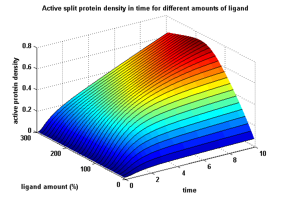 Figure 17: Split protein activity dependent on ligand amount (% of initial free receptor amount) |
Split protein activity with two different kinetic receptors
As two different receptors are used, they can differ in the kinetics. Assuming that receptor R1 is binding the ligand better, so its binding rate is higher and its dissociating rate is lower than of receptor R2. Choosing not only a higher turnover rate s1 but also a higher dimerization and a lower dimer dissociating rate for receptor R1 and a lower initial free receptor density for R2, gives the following theoretical result:
 Figure 18: Involved receptor densities in time with two different kinetic receptors involved All densities connected to R2 are shown dashed, except the dimer R1R2, which becomes the active protein. As stated in the parameters, R1 is a better binding and dimerizing receptor than R2 and is available in a higher concentration in the cell in the regarded time course. So all densities (free receptor density, monomeric density, dimeric density) connected to R1 are higher than the according densities of R2.
|
chosen parameters:
s1 = 0.2;    %turnover rate for R1
s2 = 0.1;    %turnover rate for R2
K1 = 4;      %binding rate 1
k1 = 0.05;   %dissociating rate 1
K2 = 3;      %binding rate 2
k2 = 0.1;    %dissociating rate 2
K3 = 2;      %R1R2 dimerization rate 1
k3 = 0.1;    %R1R2 dimer dissociating rate 1
K4 = 2.5;    %R1R2 dimerization rate 2
k4 = 0.05;   %R1R2 dimer dissociating rate2
K5 = 2.5;    %R1R1 dimerization rate
k5 = 0.05;   %R1R1 dimer dissociating rate
K6 = 2;      %R2R2 dimerization rate
k6 = 0.1;    %R2R2 dimer dissociating rate
Ka = 1;      %activation rate
Kda = 0.05;  %deactivation rate
initial integration conditions:
R10 = 1;     %R1
R20 = 0.7;   %R2
NN0 = 1;     %ligand
R1NN0 = 0;   %R1-Ligand monomer
R2NN0 = 0;   %R2-Ligand monomer
R1NNR20 = 0; %R1-R2 dimer
R1NNR10 = 0; %R1-R1 dimer
R2NNR20 = 0; %R2-R2 dimer
A0 = 0;      %active protein
|
 Figure 19: Split protein activity dependent on ligand amount (% of initial free receptor amount) with two different kinetic receptors involved |
Matlab m-files
 Literature Literature
- Martin F. Bachmann, Michael Salzmann, Annette Oxenius and Pamela S. Ohashi: "Formation of TCR dimers/trimers as a crucial step for T cell activation", Eur. J. Immunol., 1998
- Martin F. Bachmann and Pamela S. Ohashi: "The role of T-cell receptor dimerization in T-cell activation", Review Immunology Today, 1999
- João Sousa and Jorge Carneiro: "A mathematical analysis of TCR serial triggering and down-regulation", Eur. J. Immunol., 2000
- Susana Minguet, Mahima Swamy, Balbino Alarcón, Immanuel F. Luescher and Wolfgang W.A. Schamel: "Full Activation of the T Cell Receptor requires Both Clustering and Conformational Changes at CD3", Immunity, 2006
|  "
"


