Team:Paris/Modeling/BOB
From 2008.igem.org
(→Simplification) |
|||
| (13 intermediate revisions not shown) | |||
| Line 1: | Line 1: | ||
| - | {{Paris/ | + | {{:Team:Paris/MenuBackup}} |
| - | + | ||
| + | |||
| + | |||
<center><html><div style="color:#275D96; font-size:2em;">BOB (Based On Bibliography) Approach</div></html></center> | <center><html><div style="color:#275D96; font-size:2em;">BOB (Based On Bibliography) Approach</div></html></center> | ||
<br> | <br> | ||
| Line 128: | Line 130: | ||
* We use the classical osmosis term '''η x ( [HSL] - [HSL<sub>ext</sub>] )''' where '''η = membrane permeability x ( Surface<sub> 1cell</sub> / Volume<sub> 1cell</sub> )''' is the diffusion rate expressed in time<sup>-1</sup>. | * We use the classical osmosis term '''η x ( [HSL] - [HSL<sub>ext</sub>] )''' where '''η = membrane permeability x ( Surface<sub> 1cell</sub> / Volume<sub> 1cell</sub> )''' is the diffusion rate expressed in time<sup>-1</sup>. | ||
* The degradation rate is naturally linear: '''- γ x [HSL]'''. | * The degradation rate is naturally linear: '''- γ x [HSL]'''. | ||
| - | * To model the production, we were | + | * To model the production, we were inspired by [[Team:Paris/Modeling/BOB#Bibliography|[2]]] where it is described as being linear: '''β x [LasI]''' (β is a given constant value). However, the results presented in this study were introduced as only being theoretical and it is also possible to model the creation of HSL by a Michaelis Menten expression (similar to a Hill expression when there is no cooperativity). |
* The final expression where Θ<sub>HSL</sub> is expressed in concentration units and β<sub>HSL</sub> in (concentration * time) unit is: [[Image:HSL_final_choice_2.jpg|center]] | * The final expression where Θ<sub>HSL</sub> is expressed in concentration units and β<sub>HSL</sub> in (concentration * time) unit is: [[Image:HSL_final_choice_2.jpg|center]] | ||
| Line 153: | Line 155: | ||
=== Discussion === | === Discussion === | ||
==== Normalization ==== | ==== Normalization ==== | ||
| - | * | + | * [HSL] can be normalized for simplification purposes. According to [[Team:Paris/Modeling/BOB#Bibliography|[8]]] (table 2 of the article), at the equilibrium [HSL] can be estimated to be about 230 nM. Thresholds for TetR production (hill kinetics depending on [HSL]) become 0.160 nM -> 6.96e-4 and 0.0089 nM -> 3.87e-5 (initial values are from [[Team:Paris/Modeling/BOB#Bibliography|[4]]] and the reference value from [[Team:Paris/Modeling/BOB#Bibliography|[8]]] then becomes the 1 = 'equilibrium' value) |
* Nevertheless, it is coherent to normalize [tetR]. Likewise we set out time-scale by setting the degradation rates to the value of 1 in the previous equations, we set γ<sub>tetR</sub> to 1. Following the same train of thought as in the first subsystem, if we consider the equilibrium hypothetical stage when [HSL] concentration is fully expressed, we deduce that : | * Nevertheless, it is coherent to normalize [tetR]. Likewise we set out time-scale by setting the degradation rates to the value of 1 in the previous equations, we set γ<sub>tetR</sub> to 1. Following the same train of thought as in the first subsystem, if we consider the equilibrium hypothetical stage when [HSL] concentration is fully expressed, we deduce that : | ||
[[Image:Beta_limit_2.jpg|center]] | [[Image:Beta_limit_2.jpg|center]] | ||
| Line 186: | Line 188: | ||
<span class="keyword">function</span> output = difference(xspan,parameters) | <span class="keyword">function</span> output = difference(xspan,parameters) | ||
| - | output = parameters(1) * arrayfun(@( | + | output = parameters(1) * arrayfun(@(x)(hill(x,parameters(2),parameters(3))),xspan) - set; |
<span class="keyword">end</span> | <span class="keyword">end</span> | ||
lsqnonlin_options = optimset(<span class="string">'LevenbergMarquardt'</span>,<span class="string">'on'</span>,<span class="string">'TolX'</span>,1e-10,<span class="string">'MaxFunEvals'</span>,1e7,<span class="string">'TolFun'</span>,1e-5); | lsqnonlin_options = optimset(<span class="string">'LevenbergMarquardt'</span>,<span class="string">'on'</span>,<span class="string">'TolX'</span>,1e-10,<span class="string">'MaxFunEvals'</span>,1e7,<span class="string">'TolFun'</span>,1e-5); | ||
| Line 196: | Line 198: | ||
</pre></html> | </pre></html> | ||
| - | The script below then use this | + | The script below then use this hill_find function and the optimal_parameters it returns: |
<html><pre> | <html><pre> | ||
close, clear <span class="string">all</span> | close, clear <span class="string">all</span> | ||
| - | xspan = | + | xspan = linspace(0,1,1e4); |
| - | hillsum = 0.5 * arrayfun(@(x)(hill(x, | + | hillsum = 0.5 * arrayfun(@(x)(hill(x,6.96e-4,1) + hill(x,3.87e-5,1.5)),xspan); |
parameters = hill_find(xspan,hillsum); | parameters = hill_find(xspan,hillsum); | ||
| - | + | newhill = parameters(1)*arrayfun(@(x)(hill(x,parameters(2),parameters(3))),xspan); | |
plot(xspan,hillsum,<span class="string">'blue'</span>) | plot(xspan,hillsum,<span class="string">'blue'</span>) | ||
hold <span class="string">on</span> | hold <span class="string">on</span> | ||
| - | plot(xspan, | + | plot(xspan,newhill,<span class="string">'red'</span>) |
</pre></html> | </pre></html> | ||
| - | |||
| - | |||
[[Image:hillsum2hill.jpg|center]] | [[Image:hillsum2hill.jpg|center]] | ||
| - | + | We were, by running this script, able to compare the original function with a single hill. As you can see on the screenshot above, the difference is tiny so the approximation should not modify the dynamic behaviour of the global system. Values obtained are: '''β<sub>TetR</sub>=1.9948''', '''θ<sub>TetR-s</sub>=0.3638''' and '''n<sub>TetR-s</sub>=0.0145'''. Note that it does not have a true "meaning" but it is only a good numerical approximation to simplify 2 functions into one on the [0 1] domain. | |
| + | |||
[[Image:TetR_simplif.jpg|center]] | [[Image:TetR_simplif.jpg|center]] | ||
| Line 249: | Line 250: | ||
| Unit | | Unit | ||
| Source | | Source | ||
| + | |||
|- style="background: #dddddd;" | |- style="background: #dddddd;" | ||
| - | | style="background: #D4E2EF;" | | + | | style="background: #D4E2EF;"|γ |
| | | | ||
| - | | | + | | Degradation rate |
| - | + | ||
| - | + | ||
| - | + | ||
| - | + | ||
| - | + | ||
| - | + | ||
| - | + | ||
| - | + | ||
| - | + | ||
| - | + | ||
| - | + | ||
| - | + | ||
| - | + | ||
| - | + | ||
| - | + | ||
| - | + | ||
| - | + | ||
| - | + | ||
| - | + | ||
| - | + | ||
| - | + | ||
| - | + | ||
| - | + | ||
| - | + | ||
| 0.0198 | | 0.0198 | ||
| 1 | | 1 | ||
| min<sup>-1</sup> | | min<sup>-1</sup> | ||
| [[Team:Paris/Modeling/BOB#Remarks|wet-lab]] | | [[Team:Paris/Modeling/BOB#Remarks|wet-lab]] | ||
| - | |- style="background: #dddddd;" | + | |- style="background: #dddddd;" |
| - | | style="background: #D4E2EF;"| | + | | style="background: #D4E2EF;" |β<sub>FlhDC</sub> |
| | | | ||
| - | | | + | | Maximum production rate |
| - | | | + | | |
| 1 | | 1 | ||
| min<sup>-1</sup> | | min<sup>-1</sup> | ||
| - | | [[Team:Paris/Modeling/BOB#Remarks| | + | | [[Team:Paris/Modeling/BOB#Remarks|∅]] |
|- style="background: #dddddd;" | |- style="background: #dddddd;" | ||
| style="background: #D4E2EF;"|β<sub>FliA</sub> | | style="background: #D4E2EF;"|β<sub>FliA</sub> | ||
| Line 306: | Line 284: | ||
| min<sup>-1</sup> | | min<sup>-1</sup> | ||
| [[Team:Paris/Modeling/BOB#Bibliography|[1]]] | | [[Team:Paris/Modeling/BOB#Bibliography|[1]]] | ||
| - | |||
| - | |||
| - | |||
| - | |||
| - | |||
| - | |||
| - | |||
| - | |||
|- style="background: #dddddd;" | |- style="background: #dddddd;" | ||
| style="background: #D4E2EF;"|β<sub>CFP</sub> | | style="background: #D4E2EF;"|β<sub>CFP</sub> | ||
| Line 330: | Line 300: | ||
| min<sup>-1</sup> | | min<sup>-1</sup> | ||
| [[Team:Paris/Modeling/BOB#Bibliography|[1]]] | | [[Team:Paris/Modeling/BOB#Bibliography|[1]]] | ||
| - | |||
| - | |||
| - | |||
| - | |||
| - | |||
| - | |||
| - | |||
| - | |||
|- style="background: #dddddd;" | |- style="background: #dddddd;" | ||
| style="background: #D4E2EF;" |β<sub>YFP</sub> | | style="background: #D4E2EF;" |β<sub>YFP</sub> | ||
| Line 354: | Line 316: | ||
| min<sup>-1</sup> | | min<sup>-1</sup> | ||
| [[Team:Paris/Modeling/BOB#Bibliography|[1]]] | | [[Team:Paris/Modeling/BOB#Bibliography|[1]]] | ||
| - | |||
| - | |||
| - | |||
| - | |||
| - | |||
| - | |||
| - | |||
| - | |||
|- style="background: #dddddd;" | |- style="background: #dddddd;" | ||
| style="background: #D4E2EF;" |β<sub>RFP</sub> | | style="background: #D4E2EF;" |β<sub>RFP</sub> | ||
| Line 379: | Line 333: | ||
| [[Team:Paris/Modeling/BOB#Bibliography|[1]]] | | [[Team:Paris/Modeling/BOB#Bibliography|[1]]] | ||
|- style="background: #dddddd;" | |- style="background: #dddddd;" | ||
| - | | style="background: #D4E2EF;" | | + | | style="background: #D4E2EF;" |n<sub>envZ</sub> |
| + | | | ||
| + | | Hill coefficient | ||
| + | | | ||
| + | | 4 | ||
| + | | ¤ | ||
| + | | [[Team:Paris/Modeling/BOB#Bibliography|∅]] | ||
| + | |- style="background: #dddddd;" | ||
| + | | style="background: #D4E2EF;" |θ<sub>envZ</sub> | ||
| | | | ||
| - | | | + | | Hill characteristic concentration |
| + | | | ||
| + | | 0.5 | ||
| + | | [[Team:Paris/Modeling/BOB#Remarks|c.u]] | ||
| + | | [[Team:Paris/Modeling/BOB#Bibliography|∅]] | ||
| + | |- style="background: #dddddd;" | ||
| + | | style="background: #D4E2EF;" |β<sub>envZ</sub> | ||
| + | | | ||
| + | | Maximum production rate | ||
| + | | | ||
| + | | 1 | ||
| + | | min<sup>-1</sup> | ||
| + | | [[Team:Paris/Modeling/BOB#Remarks|∅]] | ||
| + | |- style="background: #dddddd;" | ||
| + | | style="background: #D4E2EF;" | α<sub>cell</sub> | ||
| + | | | ||
| + | | Growth rate | ||
| 0.0198 | | 0.0198 | ||
| 1 | | 1 | ||
| min<sup>-1</sup> | | min<sup>-1</sup> | ||
| [[Team:Paris/Modeling/BOB#Remarks|wet-lab]] | | [[Team:Paris/Modeling/BOB#Remarks|wet-lab]] | ||
| + | |- style="background: #dddddd;" | ||
| + | | style="background: #D4E2EF;"| c<sub>max</sub> | ||
| + | | | ||
| + | | Carrying capacity for cell growth | ||
| + | | 0.1 | ||
| + | | 0.1 | ||
| + | | µm<sup>3</sup> | ||
| + | | [[Team:Paris/Modeling/BOB#Bibliography|[3]]] | ||
| + | |- style="background: #dddddd;" | ||
| + | | style="background: #D4E2EF;"| D<sub>renewal</sub> | ||
| + | | | ||
| + | | Dilution rate | ||
| + | | 0.00198 | ||
| + | | 0.1 | ||
| + | | min<sup>-1</sup> | ||
| + | | [[Team:Paris/Modeling/BOB#Remarks|wet-lab]] ([[Team:Paris/Modeling/BOB#Bibliography|[3]]]) | ||
| + | |- style="background: #dddddd;" | ||
| + | | style="background: #D4E2EF;"| d | ||
| + | | | ||
| + | | Death rate | ||
| + | | 0.0099 | ||
| + | | 0.5 | ||
| + | | min<sup>-1</sup> | ||
| + | | [[Team:Paris/Modeling/BOB#Remarks|wet-lab]] | ||
| + | |- style="background: #dddddd;" | ||
| + | | style="background: #D4E2EF;" |γ<sub>HSL</sub> | ||
| + | | | ||
| + | | Degradation rate | ||
| + | | 0.0053 | ||
| + | | 0.2690 | ||
| + | | min<sup>-1</sup> | ||
| + | | [[Team:Paris/Modeling/BOB#Remarks|wet-lab]] | ||
| + | |- style="background: #dddddd;" | ||
| + | | style="background: #D4E2EF;"|γ<sub>HSL<sub>ext</sub></sub> <br> <br> | ||
| + | | | ||
| + | | Degradation rate | ||
| + | | 0.0106 | ||
| + | | 0.5380 | ||
| + | | min<sup>-1</sup> | ||
| + | | [[Team:Paris/Modeling/BOB#Bibliography|[6]]] | ||
|- style="background: #dddddd;" | |- style="background: #dddddd;" | ||
| style="background: #D4E2EF;" |β<sub>HSL</sub> | | style="background: #D4E2EF;" |β<sub>HSL</sub> | ||
| | | | ||
| Production rate | | Production rate | ||
| - | | 0. | + | | 0.3168 |
| - | | | + | | 16 |
| min<sup>-1</sup> | | min<sup>-1</sup> | ||
| - | | [[Team:Paris/Modeling/BOB#Bibliography| | + | | [[Team:Paris/Modeling/BOB#Bibliography|∅]] |
|- style="background: #dddddd;" | |- style="background: #dddddd;" | ||
| style="background: #D4E2EF;" |η | | style="background: #D4E2EF;" |η | ||
| | | | ||
| Diffusion rate | | Diffusion rate | ||
| - | | | + | | 10 |
| - | | | + | | 505 |
| min<sup>-1</sup> | | min<sup>-1</sup> | ||
| [[Team:Paris/Modeling/BOB#Bibliography|[2]]] | | [[Team:Paris/Modeling/BOB#Bibliography|[2]]] | ||
| - | |||
| - | |||
| - | |||
| - | |||
| - | |||
| - | |||
| - | |||
| - | |||
|- style="background: #dddddd;" | |- style="background: #dddddd;" | ||
| style="background: #D4E2EF;"|V<sub>1Cell</sub> | | style="background: #D4E2EF;"|V<sub>1Cell</sub> | ||
| Line 419: | Line 429: | ||
| [[Team:Paris/Modeling/BOB#Remarks|wet-lab]] | | [[Team:Paris/Modeling/BOB#Remarks|wet-lab]] | ||
|- style="background: #dddddd;" | |- style="background: #dddddd;" | ||
| - | | style="background: #D4E2EF;"| | + | | style="background: #D4E2EF;" |n<sub>HSL</sub> |
| | | | ||
| - | | | + | | Hill coefficient |
| - | + | ||
| - | + | ||
| - | + | ||
| - | + | ||
| - | + | ||
| - | + | ||
| | | | ||
| - | | | + | | 4 |
| - | + | ||
| - | + | ||
| - | + | ||
| - | + | ||
| - | + | ||
| - | + | ||
| - | + | ||
| - | + | ||
| - | + | ||
| - | + | ||
| - | + | ||
| - | + | ||
| - | + | ||
| - | + | ||
| - | + | ||
| - | + | ||
| - | + | ||
| - | + | ||
| - | + | ||
| - | + | ||
| - | + | ||
| - | + | ||
| - | + | ||
| - | + | ||
| - | + | ||
| - | + | ||
| - | + | ||
| - | + | ||
| - | + | ||
| - | + | ||
| - | + | ||
| - | + | ||
| - | + | ||
| - | + | ||
| - | + | ||
| - | + | ||
| - | + | ||
| - | + | ||
| - | + | ||
| - | + | ||
| - | + | ||
| - | + | ||
| - | + | ||
| - | + | ||
| - | + | ||
| - | + | ||
| - | + | ||
| - | + | ||
| - | + | ||
| - | + | ||
| - | + | ||
| - | + | ||
| - | + | ||
| - | + | ||
| - | + | ||
| - | + | ||
| - | + | ||
| - | + | ||
| ¤ | | ¤ | ||
| [[Team:Paris/Modeling/BOB#Bibliography|[3]]] | | [[Team:Paris/Modeling/BOB#Bibliography|[3]]] | ||
|- style="background: #dddddd;" | |- style="background: #dddddd;" | ||
| - | | style="background: #D4E2EF;" |θ<sub> | + | | style="background: #D4E2EF;" |θ<sub>HSL</sub> |
| | | | ||
| Hill characteristic concentration for the second operator | | Hill characteristic concentration for the second operator | ||
| - | |||
| - | |||
| - | |||
| - | |||
| - | |||
| - | |||
| | | | ||
| - | + | | 0.5 | |
| - | | 0. | + | |
| - | + | ||
| - | + | ||
| - | + | ||
| - | + | ||
| - | + | ||
| - | + | ||
| - | + | ||
| - | + | ||
| - | + | ||
| - | + | ||
| - | + | ||
| - | + | ||
| - | + | ||
| - | + | ||
| - | + | ||
| - | + | ||
| - | + | ||
| - | + | ||
| - | + | ||
| - | + | ||
| - | + | ||
| - | + | ||
| - | + | ||
| - | + | ||
| - | + | ||
| [[Team:Paris/Modeling/BOB#Remarks|c.u]] | | [[Team:Paris/Modeling/BOB#Remarks|c.u]] | ||
| - | | [[Team:Paris/Modeling/BOB#Bibliography|[ | + | | [[Team:Paris/Modeling/BOB#Bibliography|[3]]] |
| + | |||
| + | |||
|}</center> | |}</center> | ||
| Line 552: | Line 468: | ||
* [6]Lingchong You, Robert Sidney Cox III, Ron Weiss, Frances H. Arnold. ''Programmed population control by cell-cell communication and regulation killing.'' Nature, April 22, 2004. | * [6]Lingchong You, Robert Sidney Cox III, Ron Weiss, Frances H. Arnold. ''Programmed population control by cell-cell communication and regulation killing.'' Nature, April 22, 2004. | ||
* [7] Braun D et al. ''Parameter Estimation for Two Synthetic Gene Networks: A Case Study'', ICASSP 5:769-772, 2005. | * [7] Braun D et al. ''Parameter Estimation for Two Synthetic Gene Networks: A Case Study'', ICASSP 5:769-772, 2005. | ||
| - | + | * [8] Pearson et al. ''Active Efflux and Diffusion Are Involved in Transport of Pseudomonas aeruginosa Cell-to-Cell Signals'' Journal of Bacteriology, February 1999, p. 1203-1210, Vol. 181, No. 4 | |
<center>[[Team:Paris/Modeling/BOB#Introduction|Back to the top of the page]]</center> | <center>[[Team:Paris/Modeling/BOB#Introduction|Back to the top of the page]]</center> | ||
| - | |||
|} | |} | ||
Latest revision as of 04:46, 30 October 2008
Go back to the normal Wiki
Contents |
Introduction
- The key problem with a dynamic system consists in the fact that adding a new equation gives a more detailed idea of the overall process, but one looses meaning by doing so since new undefined parameters appear. Hence, it becomes hard to link those parameters with a biological meaning and reality.
- In that respect we chose to build at first a simplified model, which would enable us to help us understand the processes implied in the system. In that respect, we chose not to introduce the mRNA state between transcription and translation in our model. We presented things as if a protein would act directly upon the following. Furthermore, we assumed that describing routinely every step, would only force us into finding more parameters.
- This preliminary approach is mainly based on a bibliographical work. In fact, it is important to understand that with this approach, we did not intend to design the most accurate model possible. We found essential to choose only parameters that we could determine or control in the wet lab. The main goal was to get quickly a first idea of the way our system could behave.
- The goal here is to present the differential equations we used in the model. At each step we shall describe why we chose these precise equations, the drawbacks and possible improvements, the parameters involved and eventually a biologically coherent value.
Model
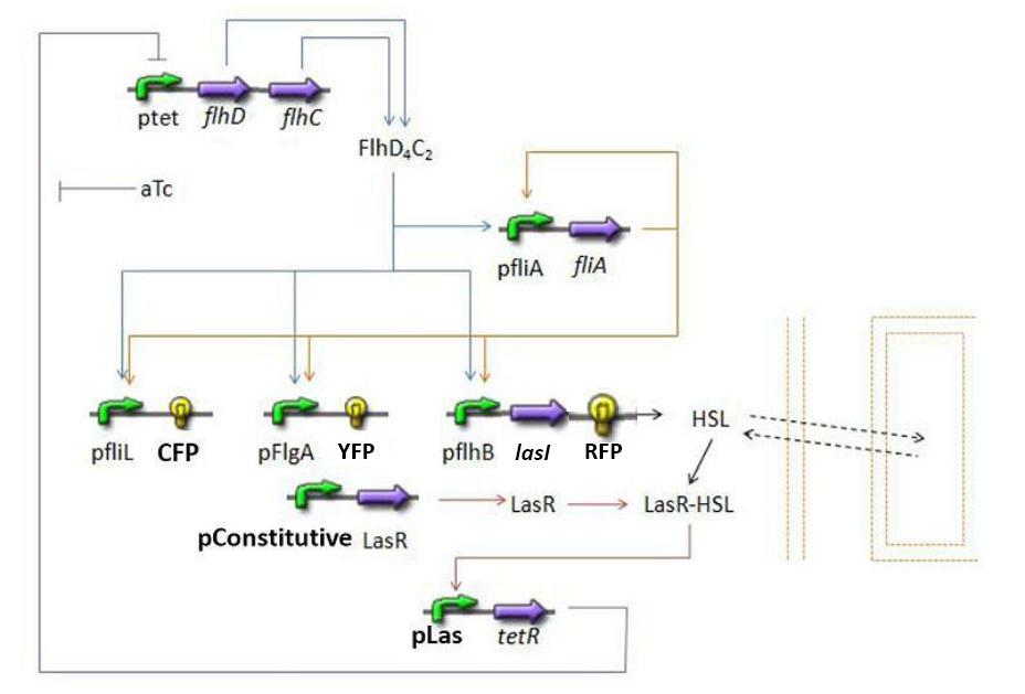
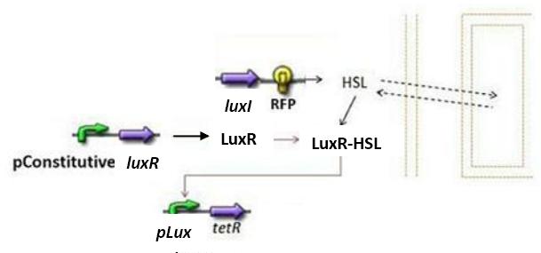
- Here is an overall view of the whole system :
Steps of the Model
We chose to broke up this system in three sub systems for presentation clarity
- Population Growth : we wished to model the population evolution in the chemostat, since our experiments will be carried out in these conditions.
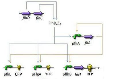
- First Subsystem
- FliA behind pFliA= f(FlhDC,FliA)
- CFP behind pFliL = f(FlhDC,FliA)
- YFP behind pFlgA = f(FlhDC,FliA)
- RFP and LasI behind pFlhB = f(FlhDC,FliA)
(See also our FIFO module and the Simulation of the FIFO)
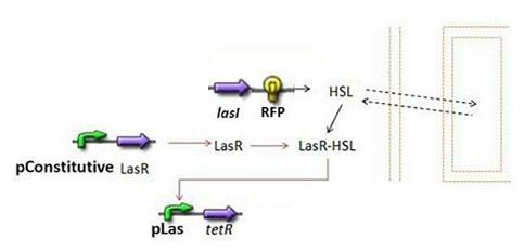
- Second Subsystem
- HSL = f(LasI) or f(LuxI) depending on which system is being used
- HSL ⇋ HSLext
- TetR = f(HSL)
(See also our Synchronisation module)
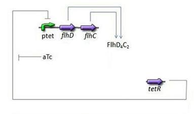
- Third Subsystem
- FlhDC = f(TetR)
- In each subsystem we will describe the way we decided to normalize each protein resulting from genic expression. In fact, in every case we normalize the concentration by their maximum values, in order to keep the influence relations that rule the system behavior. This will enable us to compare the different concentration evolutions, and interpret the data we get from our simulations.
Population evolution
- First of all, it seems important at this stage to present the way we interpret the evolution of the population in the chemostat. We want to impose to our model the fact that the rate of production has to be proportional to the existing population and to the amount of available resources. Hence a logistic model of the population, where c denotes the concentration of cells in the medium:
- Then, we need to add the death term, and a dilution term cause by the renewal of the chemostat. Finally we get :
where cmax is the carrying capacity for cell growth, and
![]() the dilution rate, d the death rate constant
the dilution rate, d the death rate constant
First Subsystem
Steps involved
- FliA behind pFliA= f(FlhDC,FliA)
- CFP behind pFliL = f(FlhDC,FliA)
- YFP behind pFlgA = f(FlhDC,FliA)
- RFP and LasI behind pFlhB = f(FlhDC,FliA)
Mathematical model
- Classically we use the following equation to model gene interactions (see for example in [5]) :
where [Y] denotes the concentration of Y protein and γ its degradation rate (which unit is time-1).
- Yet, the flagella gene network has been thoroughly studied in [1]. We used two major results presented in this study. Firstly, Shiraz Kalir and Uri Alon came up with the fact that the promoters of class 2 genes, among which fliL, flgA and flhB, behaved like SUM-gate functions with flhDC and fliA inputs. Secondly, their experiments proved that these influences could be considered as linear. Thus the following model:
β and β’ represent the relative influence of flhDC and fliA respectively, the units of β and β’ being time-1.
- Furthermore, they came up with numerical values of β and β’ for each gene, which fitted quite well to their experiments. We then decided that we could use those values as well in our model.
- Finally, here are our final equations:
Discussion
Normalization
- First of all, we wanted to have a proper time scale. We the set the degradation rates, γ ,to 1. It is important to note that this degradation rate represents the influence of the degradation and dilution. We assume that the degradation can be neglected compared to the dilution caused by the cell growth. Then we have:
- Since we can know easily the value of the real half-time, we may know the real timescale out of our computations. We kept the designation “degradation rate” for convenience, so as not to mix up with the dilution that occurs with the HSL in the synchronisation step.
- We kept the β and β’ values found by S. Kalir and U. Alon, since they showed the relative influence of flhDC and fliA. To have the same order of magnitude between each specie, we normalized those parameters between 0 and 1 as following. We reasoned independently for each equation, wishing to set the equilibrium values of the concentration to 1 given input values of 1. This gave:
- In fact, if we take CFP for example:
The maximum of [CFP] is reached when [fliA] = 1 and [flhDC] = 1 ; when we solve with these condidtions, we obtain :
Then setting the equilibrium value of [CFP] to 1 corresponds to setting
- The analysis of fliA is different, but not the result:
With an input of flhDC equal to 1, the solution of the differential equation is:
And the condition on the equilibrium imposes
- To conclude, we see that we always get the same condition:
- Finally, since we had imposed γ=1 we resulted with β+β'=1.
Which gene goes were?
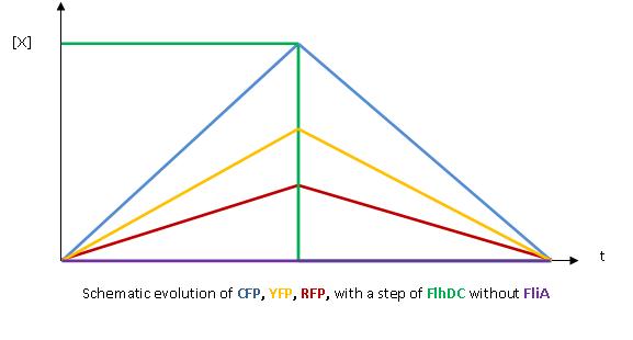
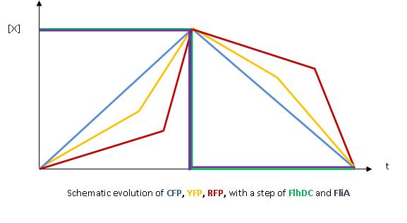
- The key element to understand is that fliA stands as an accelerator. The first influence is caused by flhDC, and fliA gives the last burst. fliA also has a great influence in the fading phase, since it introduces a delay (result found by experiments in [1]). This is what determined our choice in the order of fliL, flgA and flhB. We wanted to put in first the gene that was the least influenced by fliA, and in the end the gene the most influenced by fliA.
- We wished to run simulations with Matlab to confirm this reasoning : for further information see our simulations.
- In fact, this enabled us to force the curves into crossing themselves. In addition, the delay imposed by fliA in the decreasing phase, would permit us to widen the delays between the first and the last gene expression, thus getting better conditions to observe the FIFO in the wet lab.
Second Subsystem
Steps involved
- HSL = f(LasI) or f(LuxI) depending on which system is being used
- HSL ⇋ HSLext
- TetR = f(HSL)
Mathematical Model
Dynamics of HSL
- First and foremost, it is clear that HSL is the key element in the synchronisation process: we used a diffusive specie in order to insert a reference specie inside the medium. Therefore, the HSL concentration, denoted [HSL], is the link to the outside medium HSL concentration, denoted [HSLext], which is the intermediate reference value.
- We use the classical osmosis term η x ( [HSL] - [HSLext] ) where η = membrane permeability x ( Surface 1cell / Volume 1cell ) is the diffusion rate expressed in time-1.
- The degradation rate is naturally linear: - γ x [HSL].
- To model the production, we were inspired by [2] where it is described as being linear: β x [LasI] (β is a given constant value). However, the results presented in this study were introduced as only being theoretical and it is also possible to model the creation of HSL by a Michaelis Menten expression (similar to a Hill expression when there is no cooperativity).
- The final expression where ΘHSL is expressed in concentration units and βHSL in (concentration * time) unit is:
- It is important to note that we took into account the fact that lasR/(lasR linked to HSL) was a function of HSL. However, we assumed that the fraction of HSL bound to lasR would not influence HSL concentration; this is the reason why, no "degradation due to binding" term appears in the HSL model.
- Last but not least, lasR does not intervene in the equations because we have considered it to be constitutively expressed. Like aTc (see below), it can be used later as a control for our system.
Dynamics of HSLext
- The evolution of HSLext may be described with three terms. First of all, there is a dilution rate, Drenewal, due to the renewal of the chemostat. There is the usual degradation rate,γ[HSL]ext. Then we have a the osmotic term, likewise the one presented before :
- If [HSL]ext > [HSL], then there is a positive flow of HSL from inside the cells to the exterior medium.
- Else, if[HSL]ext < [HSL], then there is a negative flow of HSL (from outside to inside the cells).
Which gives
where
TetR=f(HSL)
- Here we had the choice to model the complexation phase of HSL and lasR, and then the binding phase of this complex on the pLas promoter. We assumed that those stages were fast, and then decided to model them by a single step.
- We checked in the registry that the pLas sequence was the same as the one of lasB described in [4]. It is explained that there are two operators, denoted OP1 and OP2. The Hill parameters were detailed in this article, hence our modeling choice:
- It is noticeable that we assumed a "sum" behavior for the two operons.
Discussion
Normalization
- [HSL] can be normalized for simplification purposes. According to [8] (table 2 of the article), at the equilibrium [HSL] can be estimated to be about 230 nM. Thresholds for TetR production (hill kinetics depending on [HSL]) become 0.160 nM -> 6.96e-4 and 0.0089 nM -> 3.87e-5 (initial values are from [4] and the reference value from [8] then becomes the 1 = 'equilibrium' value)
- Nevertheless, it is coherent to normalize [tetR]. Likewise we set out time-scale by setting the degradation rates to the value of 1 in the previous equations, we set γtetR to 1. Following the same train of thought as in the first subsystem, if we consider the equilibrium hypothetical stage when [HSL] concentration is fully expressed, we deduce that :
and solving gives:
thus the conclusion :
Concerning the Lux system
- We shall try to construct both systems (las and lux). In the case of the lux system, the only change would be in the expression of TetR. Indeed, since there is a single operator we have modeled [TetR] dynamics as follows, reasoning like in the las system :
- Concerning the normalization, according to the previous reasoning, we have βTetR(lux)=1.
Simplification
In our system, HSL activates the pLas promoter which control the transcription of tetR. According to the bibliography the pLas promoter is made of two distincts operators, each operator's action being modeled by a Hill function as explained above.
However, to simplify the global model, we wanted to keep only linear or hill activation but not mixed expressions like a sum of two hill functions. Any function can be approximated by another but the square difference will of course become important if you don't choose the new function and its parameters accurately.
To sum up, we had to simplify βTetR x ( hill(x , θTetR-OP1 , nTetR-OP1) + hill(x , θTetR-OP2 , nTetR-OP2) ) by something more consistant with the model. We chose to use a single hill function 0.5 x βTetR x hill(x,θTetR-s,nTetR-s), still having to find the new threshold and steepness parameters (subscripted -s).
It is an optimization issue which can be solved by the lsqnonlin Matlab function. The following function that we wrote can find the parameters of the hill function that fit the best to a given timespan and set of points:
function optimal_parameters = hill_find(xspan,set)

function output = difference(xspan,parameters)
output = parameters(1) * arrayfun(@(x)(hill(x,parameters(2),parameters(3))),xspan) - set;
end
lsqnonlin_options = optimset('LevenbergMarquardt','on','TolX',1e-10,'MaxFunEvals',1e7,'TolFun',1e-5);
optimal_parameters = lsqnonlin(@(parameters)difference(xspan,parameters), ...
[1 1 1],[0 0 0],[10 10 10],lsqnonlin_options);
optimal_parameters = optimal_parameters(:);

end
The script below then use this hill_find function and the optimal_parameters it returns:
close, clear all

xspan = linspace(0,1,1e4);
hillsum = 0.5 * arrayfun(@(x)(hill(x,6.96e-4,1) + hill(x,3.87e-5,1.5)),xspan);
parameters = hill_find(xspan,hillsum);
newhill = parameters(1)*arrayfun(@(x)(hill(x,parameters(2),parameters(3))),xspan);

plot(xspan,hillsum,'blue')
hold on
plot(xspan,newhill,'red')
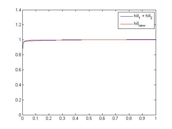
We were, by running this script, able to compare the original function with a single hill. As you can see on the screenshot above, the difference is tiny so the approximation should not modify the dynamic behaviour of the global system. Values obtained are: βTetR=1.9948, θTetR-s=0.3638 and nTetR-s=0.0145. Note that it does not have a true "meaning" but it is only a good numerical approximation to simplify 2 functions into one on the [0 1] domain.
Third Subsystem
Mathematical Model
- FlhDC = f(TetR)
- Here we chose to understand aTc as a regulation and control variable, that will help us influence our parameters in the wet lab. Therefore, [aTc] does not appear in this model.
- For this last step, in addition to the usual degradation term, we simply chose a complete Hill function to describe the dynamics of flhDC, because this is the way it is commonly described in the literature:
Discussion : Normalization
- Likewise the previous analysis, we set γFlhDC to 1. Then, since FlhDC is fully expressed when TetR is not, we see that when solving under this conditions, we get
hence the need to set
- Furthermore, since [TetR] has been normalized, we have to do so for θFlhDC as well, since its role is to stand as a reference concentration for [TetR]. Therefore, we have to normalize it in the same way we did for [TetR]:
Parameters summary
Parameters Table
| Parameter Table | ||||||
|---|---|---|---|---|---|---|
| Parameter | Parameter in code | Meaning | Original Value | Normalized Value | Unit | Source
|
| γ | Degradation rate | 0.0198 | 1 | min-1 | wet-lab | |
| βFlhDC | Maximum production rate | 1 | min-1 | ∅ | ||
| βFliA | FlhDC activation coefficient | 50 | 0.1429 | min-1 | [1] | |
| β'FliA | FliA activation coefficient | 300 | 0.8571 | min-1 | [1] | |
| βCFP | FlhDC activation coefficient | 1200 | 0.8276 | min-1 | [1] | |
| β'CFP | FliA activation coefficient | 250 | 0.1724 | min-1 | [1] | |
| βYFP | FlhDC activation coefficient | 150 | 0.3333 | min-1 | [1] | |
| β'YFP | FliA activation coefficient | 300 | 0.6667 | min-1 | [1] | |
| βRFP | FlhDC activation coefficient | 100 | 0.2222 | min-1 | [1] | |
| β'RFP | FliA activation coefficient | 350 | 0.7778 | min-1 | [1] | |
| nenvZ | Hill coefficient | 4 | ¤ | ∅ | ||
| θenvZ | Hill characteristic concentration | 0.5 | c.u | ∅ | ||
| βenvZ | Maximum production rate | 1 | min-1 | ∅ | ||
| αcell | Growth rate | 0.0198 | 1 | min-1 | wet-lab | |
| cmax | Carrying capacity for cell growth | 0.1 | 0.1 | µm3 | [3] | |
| Drenewal | Dilution rate | 0.00198 | 0.1 | min-1 | wet-lab ([3]) | |
| d | Death rate | 0.0099 | 0.5 | min-1 | wet-lab | |
| γHSL | Degradation rate | 0.0053 | 0.2690 | min-1 | wet-lab | |
| γHSLext | Degradation rate | 0.0106 | 0.5380 | min-1 | [6] | |
| βHSL | Production rate | 0.3168 | 16 | min-1 | ∅ | |
| η | Diffusion rate | 10 | 505 | min-1 | [2] | |
| V1Cell | Cell Volume | 1 | 1 | µm3 | wet-lab | |
| nHSL | Hill coefficient | 4 | ¤ | [3] | ||
| θHSL | Hill characteristic concentration for the second operator | 0.5 | c.u | [3]
| ||
Remarks
- We denote by c.u the arbitrary (due to normalization) concentration unit.
- We evaluated in the wet lab the half life time for our cells, and then calculated the degradation constants using :
The value for half-life time we found and used is 35min.
- Furthermore, Drenewal is a wet-lab data since we can impose the exact value of our wish. What is more, thanks to this model, we are able to evaluate an optimised value of this parameter so as to carry the experiments with the best probability to have the wanted behavior.
- ∅ occurance in the table corresponds to value we did not need due to our normalization process.
Bibliography
Much of our inspiration comes from four articles to which we shall refer in the next subsections :
- [1] Shiraz Kalir, Uri Alon. Using quantitative blueprint to reprogram the dynamics of the flagella network. Cell, June 11, 2004, Vol.117, 713-720.
- [2]Jordi Garcia-Ojalvo, Michael B. Elowitz, Steven H. Strogratz. Modeling a synthetic multicellular clock : repressilators coupled by quorum sensing. PNAS, July 27, 2004, Vol. 101, no. 30.
- [3]Frederick K. Balagaddé, Hao Song, Jun Ozaki, Cynthia H. Collins, Matthew Barnet, Frances H. Arnold, Stephen R. Quake, Lingchong You. A Synthetic Escherichia Coli predator prey ecosystem. Molecular Systems Biology. 2008.
- [4]M. Schuster, M. L Urbanowski, E. P. Greenberg. Promoter Specificity in Pseudomonas aeruginosa quorum sensing revealed by DNA binding of purified LasR. PNAS, November 9, 2004, vol. 101, no. 45.
- [5]Nitzan Rosenfeld, Michael B. Elowitz, Uri Alon. Negative autoregulation speeds the response times of transcription networks. JMB, 2003, 323, 785-793.
- [6]Lingchong You, Robert Sidney Cox III, Ron Weiss, Frances H. Arnold. Programmed population control by cell-cell communication and regulation killing. Nature, April 22, 2004.
- [7] Braun D et al. Parameter Estimation for Two Synthetic Gene Networks: A Case Study, ICASSP 5:769-772, 2005.
- [8] Pearson et al. Active Efflux and Diffusion Are Involved in Transport of Pseudomonas aeruginosa Cell-to-Cell Signals Journal of Bacteriology, February 1999, p. 1203-1210, Vol. 181, No. 4
|}
 "
"

