Team:Heidelberg/Notebook/Visualization/Methods
From 2008.igem.org
(→computer-assisted analysis) |
(→chemotactical activity) |
||
| (41 intermediate revisions not shown) | |||
| Line 463: | Line 463: | ||
</html> | </html> | ||
| - | '''Visualization - Methods revealed''' | + | '''Visualization - Methods revealed'''<br> |
| + | [https://2008.igem.org/Team:Heidelberg/Notebook/visualization '''back to the visualization notebook''']<br> | ||
| - | = | + | =Microscopy= |
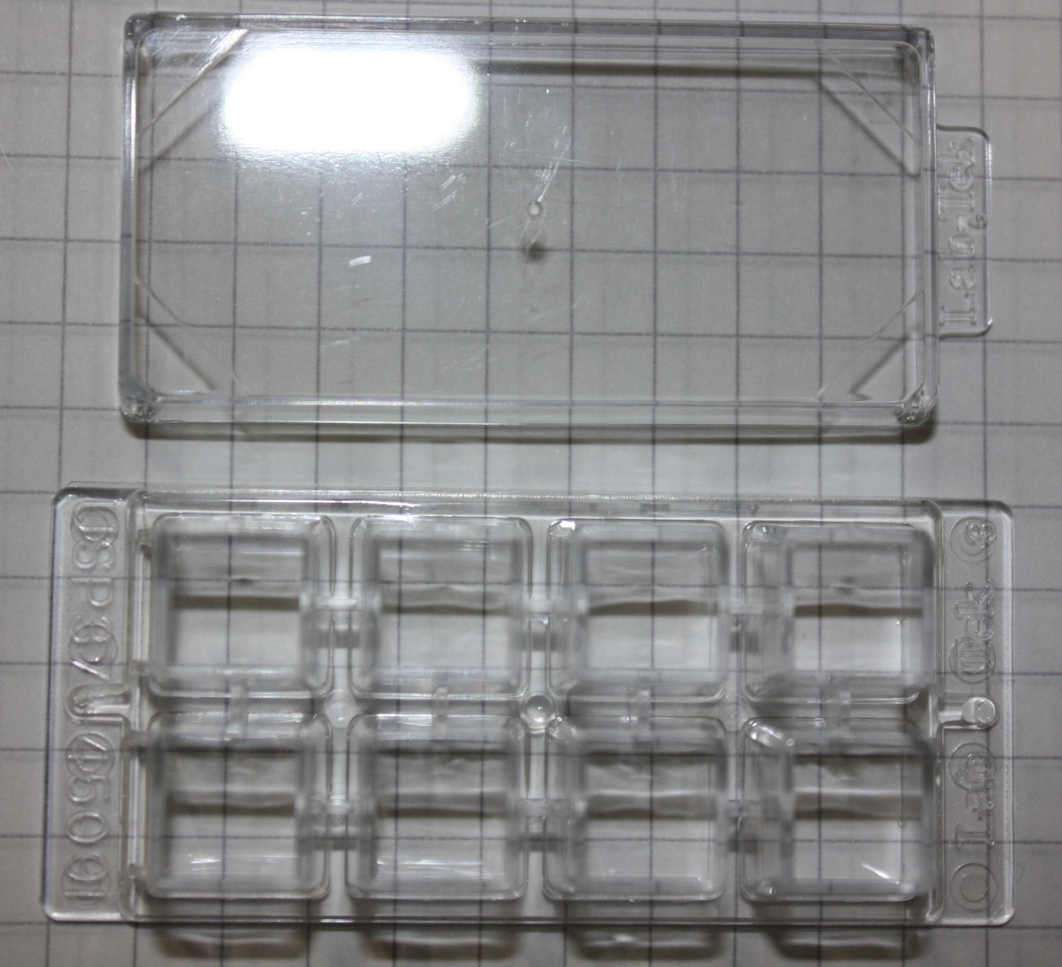
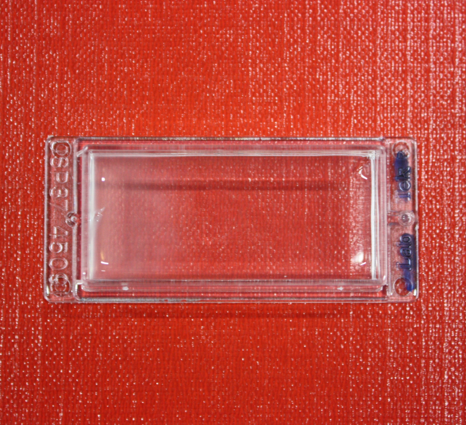
| - | Was performed using LabtekTM | + | Was performed using LabtekTM chambers (Nunc, Rochester, NY, USA) in two formats: |
| - | + | ||
[[Image:Small_chamber.jpg|left|thumb|200px|Small chamber 2x4 wells]][[Image:Large_chamber.jpg|left|thumb|200px|Large chamber]] | [[Image:Small_chamber.jpg|left|thumb|200px|Small chamber 2x4 wells]][[Image:Large_chamber.jpg|left|thumb|200px|Large chamber]] | ||
| Line 474: | Line 474: | ||
<br><br><br><br><br><br><br><br><br><br><br><br><br> | <br><br><br><br><br><br><br><br><br><br><br><br><br> | ||
| - | + | Samples were monitored using an Applied Precision - DeltaVision wide field microscope. | |
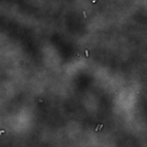
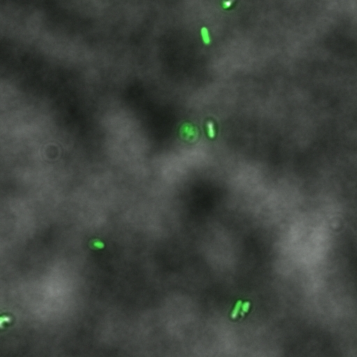
| - | After the first experiments have been | + | After the first experiments have been done in bright-field mode, further experiments were only performed with fluorescent strains. They are much more accurate and are much more suitable for quantitative analysis methods. |
[[Image:usual_trans_photo.jpg|left|thumb|150px|Usual transmission]][[Image:making_them_fluorescent.jpg|left|thumb|150px|Merged picture]][[Image:more_accurate.jpg|left|thumb|150px|Fluorescent shot]] | [[Image:usual_trans_photo.jpg|left|thumb|150px|Usual transmission]][[Image:making_them_fluorescent.jpg|left|thumb|150px|Merged picture]][[Image:more_accurate.jpg|left|thumb|150px|Fluorescent shot]] | ||
| Line 481: | Line 481: | ||
<br><br><br><br><br><br><br><br><br><br><br> | <br><br><br><br><br><br><br><br><br><br><br> | ||
| - | + | [https://2008.igem.org/Team:Heidelberg/Notebook/Visualization/Methods back up] | |
==Frames== | ==Frames== | ||
| - | [[Image:smallframe.jpg|right|thumb|300px|Sample of a frame used for small chambers]][[Image:bigframe.jpg|right|thumb|200px| | + | [[Image:smallframe.jpg|right|thumb|300px|Sample of a frame used for small chambers]][[Image:bigframe.jpg|right|thumb|200px|Illustration of two frames on a large chamber, each frame is covering one half of the chamber]] |
<br> | <br> | ||
| - | To analyse chamber samples | + | To analyse chamber samples at several time points (''e.g. after 3,6,9 hours ...'')<br> under the microscope a regular pattern for image acquisition was needed. Therefore several frames have been developed, which cover the chamber as good as possible and give the best insights into the events of the experiment. |
| - | Therefore several frames have been developed, which cover the chamber as good as possible and | + | |
On the right side is one example for each type of chamber: | On the right side is one example for each type of chamber: | ||
Every black spot stands for a taken picture at this position.<br> | Every black spot stands for a taken picture at this position.<br> | ||
| - | + | The rectangles are just examples of potential frames. | |
| - | For small chambers square frames were used like 10x10 or 8x8 | + | For small chambers square frames were used like 10x10 or 8x8, resulting in 100 or 64 pictures in total. |
| - | To cover | + | To cover the complete area of a large chamber two separate frames had to be used. Each of those frames contained 6x8 (6 in height and 8 in width) images. |
<br><br><br><br><br><br><br> | <br><br><br><br><br><br><br> | ||
| - | + | [https://2008.igem.org/Team:Heidelberg/Notebook/Visualization/Methods back up] | |
==chemotactical activity== | ==chemotactical activity== | ||
[[Image:chemoactivity.jpg|right|thumb|300px|]] | [[Image:chemoactivity.jpg|right|thumb|300px|]] | ||
| - | This test | + | This test series was used to test the chemotactic activity of strains depending on special strain abilities and the media they were incubated in or transferred to. |
3 µl of an overnight culture were put into a small chamber filled with 200 µl of the appropriate media. <br> | 3 µl of an overnight culture were put into a small chamber filled with 200 µl of the appropriate media. <br> | ||
| - | The | + | The activity of the bacteria has been observed over several hours. Depending on the experiment sometimes after a specific time an attractant like casamino acids has been added to the media to test the effect of the attractant on the activity of the specific strain. |
<br><br> | <br><br> | ||
This was performed with short time lapse series like taking 90 pictures at one position with a time lapse of less than 0.33 seconds. | This was performed with short time lapse series like taking 90 pictures at one position with a time lapse of less than 0.33 seconds. | ||
<br><br> | <br><br> | ||
This experiment may give an idea of the behavior of certain strains under specific conditions.<br> | This experiment may give an idea of the behavior of certain strains under specific conditions.<br> | ||
| - | With this information it is | + | With this information it is easier to choose the right strain and the best conditions for further experiments.<br> |
| - | It is also possible to predict the bacterial behavior, so that some parameters can be excluded if the bacteria do not act as expected. | + | It is also possible to predict the bacterial behavior, so that some parameters can be excluded, if the bacteria do not act as expected. |
<br><br> | <br><br> | ||
| - | Here is one example of such a time lapse serie: | + | Here is one example of such a time lapse serie:<br> |
| + | ''To see this video the quicktime plugin for the appropriate browser is needed. The [http://www.apple.com/de/quicktime/download/ Quicktime] player is freely available and can be downloaded from apple.com '' | ||
<html> | <html> | ||
<center> | <center> | ||
| - | <embed src="https://static.igem.org/mediawiki/2008/6/6b/Chemo_HCB33_20080917_LB_05OD_1h_R3D.avi.MOV" width= | + | <embed src="https://static.igem.org/mediawiki/2008/6/6b/Chemo_HCB33_20080917_LB_05OD_1h_R3D.avi.MOV" width=400px height=360px loop=true></embed> |
</center> | </center> | ||
</html> | </html> | ||
| - | + | [https://2008.igem.org/Team:Heidelberg/Notebook/Visualization/Methods back up] | |
==computer-assisted analysis== | ==computer-assisted analysis== | ||
| + | ===ImageJ=== | ||
| - | The Deltavision | + | The Deltavision wide field microscope creates Deltavision files (.dv) as output, which may be in stacks or not colored as wanted. To automatically convert the vast amount of generated .dv files into Jpeg files and to process the images, homemade plugins for ImageJ were used. (''For example by coloring and/or merging.'')<br> |
| - | + | ||
| - | + | For the automatic processing an importer plugin [http://www.loci.wisc.edu/ome/formats-imagej.html LOCI Bio-Formats] was used. The link can be found by clicking on the name.<br> | |
| - | This plugin enables the automatic processing of Deltavision | + | This plugin enables the automatic processing of Deltavision files into ImageJ. |
An example for such a plugin would be: | An example for such a plugin would be: | ||
[[Image:Convertandmerge.jpg|left|100px|]] | [[Image:Convertandmerge.jpg|left|100px|]] | ||
| - | Just click on the picture to see the plugin. | + | <br><br><br> |
| + | ''Just click on the picture above to see the plugin.'' | ||
| + | <br><br> | ||
| + | The plugin *.txt has to be in the macros folder which is located in the ImageJ mainfolder, then the plugin can be run from windows with the following command in the commandline:<br> | ||
| + | java -jar ij.jar -batch ''nameoftheplugin'' | ||
| + | |||
This plugin takes a serie of 64 pictures taken with the Deltavision microscope in the specific folder.<br> | This plugin takes a serie of 64 pictures taken with the Deltavision microscope in the specific folder.<br> | ||
| - | Each file was a stack of 2 pictures with | + | Each file was a stack of 2 pictures with two different channels. The plugin opens the files merges them to one RGB picture, converts them to Jpeg and saves the new pictures in the same folder.<br><br> |
| - | + | Those grey pictures are 2 pictures forming one stack, the third one is the product of the plugin: | |
| - | + | ||
| - | [[https://2008.igem.org/Team:Heidelberg/Notebook/Visualization/Methods back up | + | [[Image:20081024_col_kill_6h_24_R3D11.jpg|left|150px|]] [[Image:20081024_col_kill_6h_24_R3D12.jpg|left|150px|]] [[Image:20081024_col_kill_6h_24.jpg|left|150px|]] |
| + | <br><br><br><br><br><br><br><br><br> | ||
| + | |||
| + | ===Analysis with MatLab=== | ||
| + | |||
| + | Furthermore every picture can be correlated with an intensity value.<br> | ||
| + | In combination with an automatic picture arrangement function, which many image processing programs provide, it is possible to create 3D graphics, which can be compared with their frame pictures.<br> | ||
| + | To see some results of this image processing and analysis: ~~[https://2008.igem.org/Team:Heidelberg/Project/Visualization click here]~~<br> | ||
| + | <br><br> | ||
| + | An example of analysing the left frame of an experiment with the large chamber: | ||
| + | |||
| + | [[Image:MatLabanalysis.jpg|left|100px|]] | ||
| + | <br><br><br><br><br> | ||
| + | ''Just click on the picture above to see the code.'' | ||
| + | <br><br> | ||
| + | There are several other possibilities to change the calculation of the parameters and adjust the 3D graphic. | ||
| + | <br><br> | ||
| + | This can be combined with analysing the right frame as well.<br> | ||
| + | If the result like here would be A=feld and if the result of the right frame is B=feld both frames can be combined and shown as a 3D grapic with the following commands:<br><br> | ||
| + | ''C=[A,B]''<br> | ||
| + | ''surf(C')''<br> | ||
| + | ''shading interp''<br> | ||
| + | <br> Examples of this can be seen on the ''click here'' link above.<br><br> | ||
| + | [https://2008.igem.org/Team:Heidelberg/Notebook/Visualization/Methods back up] | ||
=Swarm Assays= | =Swarm Assays= | ||
| Line 551: | Line 578: | ||
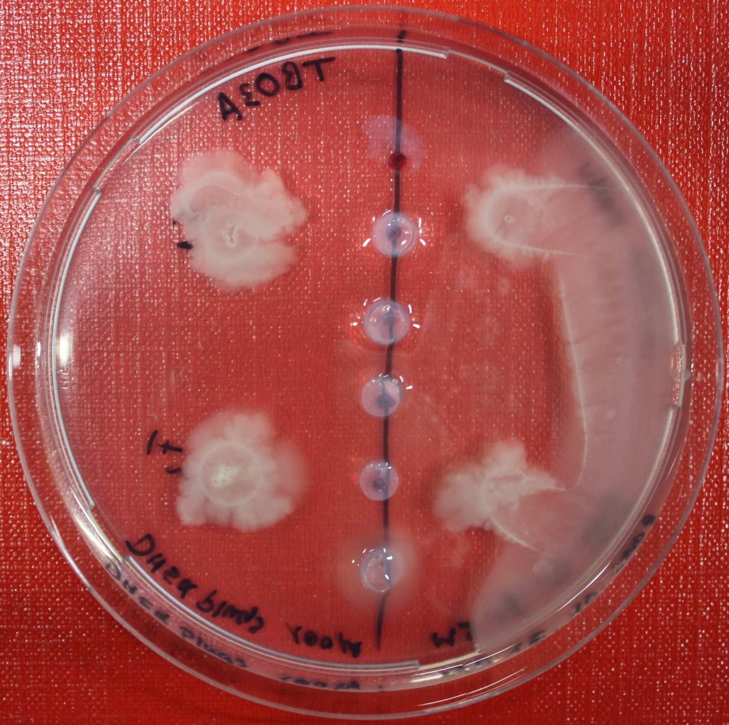
*Step 1: Make sure you have everything ready to get started. You need: | *Step 1: Make sure you have everything ready to get started. You need: | ||
| - | ** Petri-dishes. '''!!!''' ''sign your petri-dishes before You pour in the media. Also mark the spots where you want to set the attractant or attractant line and the bacteria.'' '''!!!''' | + | ** Petri-dishes. '''!!!''' ''sign your petri-dishes before You pour in the media. Also mark the spots where you want to set the attractant or attractant line and the bacteria.'' '''!!!''' Handle the soft agar with care. After the addition of the attractant the petri-dish should only be moved really carefully. |
** 50 ml falcons | ** 50 ml falcons | ||
** 25 ml media containig 0.2%-0.3% Agar for every petri-dish. | ** 25 ml media containig 0.2%-0.3% Agar for every petri-dish. | ||
** samples of the appropriate attractants. The concentration depends on several substance depending attributes. | ** samples of the appropriate attractants. The concentration depends on several substance depending attributes. | ||
** Other substances like antibiotics (Amp, Kan, Cm) or inducer (IPTG, Arabinose) | ** Other substances like antibiotics (Amp, Kan, Cm) or inducer (IPTG, Arabinose) | ||
| - | *Step 2: Your agar-media solution should be clear and the agar completely | + | *Step 2: Your agar-media solution should be clear and the agar completely dissolved. ''If you want to use attractant plugs<sup>1</sup> or other non fluid attractants, go first through step 5 then back through 2,3,4 skip 5, further with 6 and so on...'' |
*Step 3: Take Take a 50 ml falcon pour 25 ml of your agar containing media in it and add antibiotics or inducing substances. ''If no extra substances are needed just skip this step.'' | *Step 3: Take Take a 50 ml falcon pour 25 ml of your agar containing media in it and add antibiotics or inducing substances. ''If no extra substances are needed just skip this step.'' | ||
*Step 4: Let your media polimerize. At least let it rest for 15/20 min. | *Step 4: Let your media polimerize. At least let it rest for 15/20 min. | ||
| Line 575: | Line 602: | ||
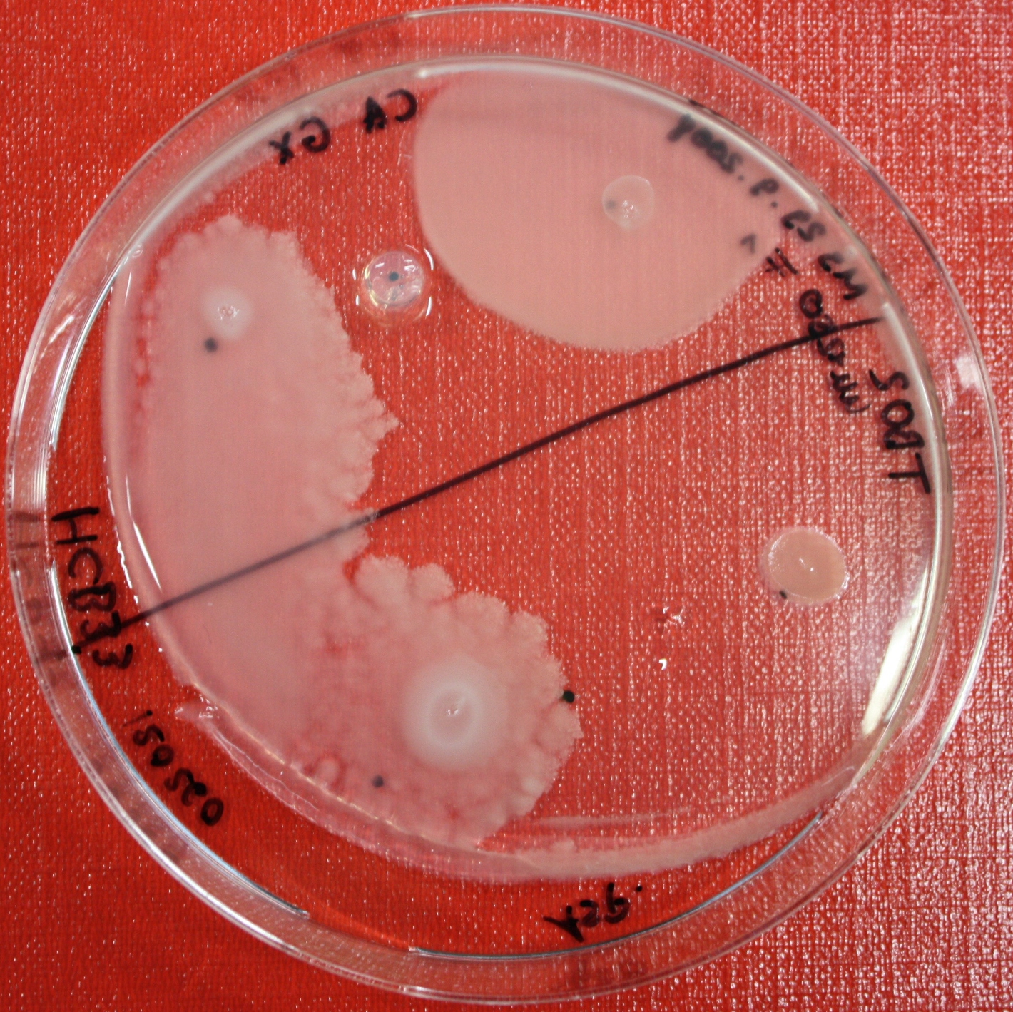
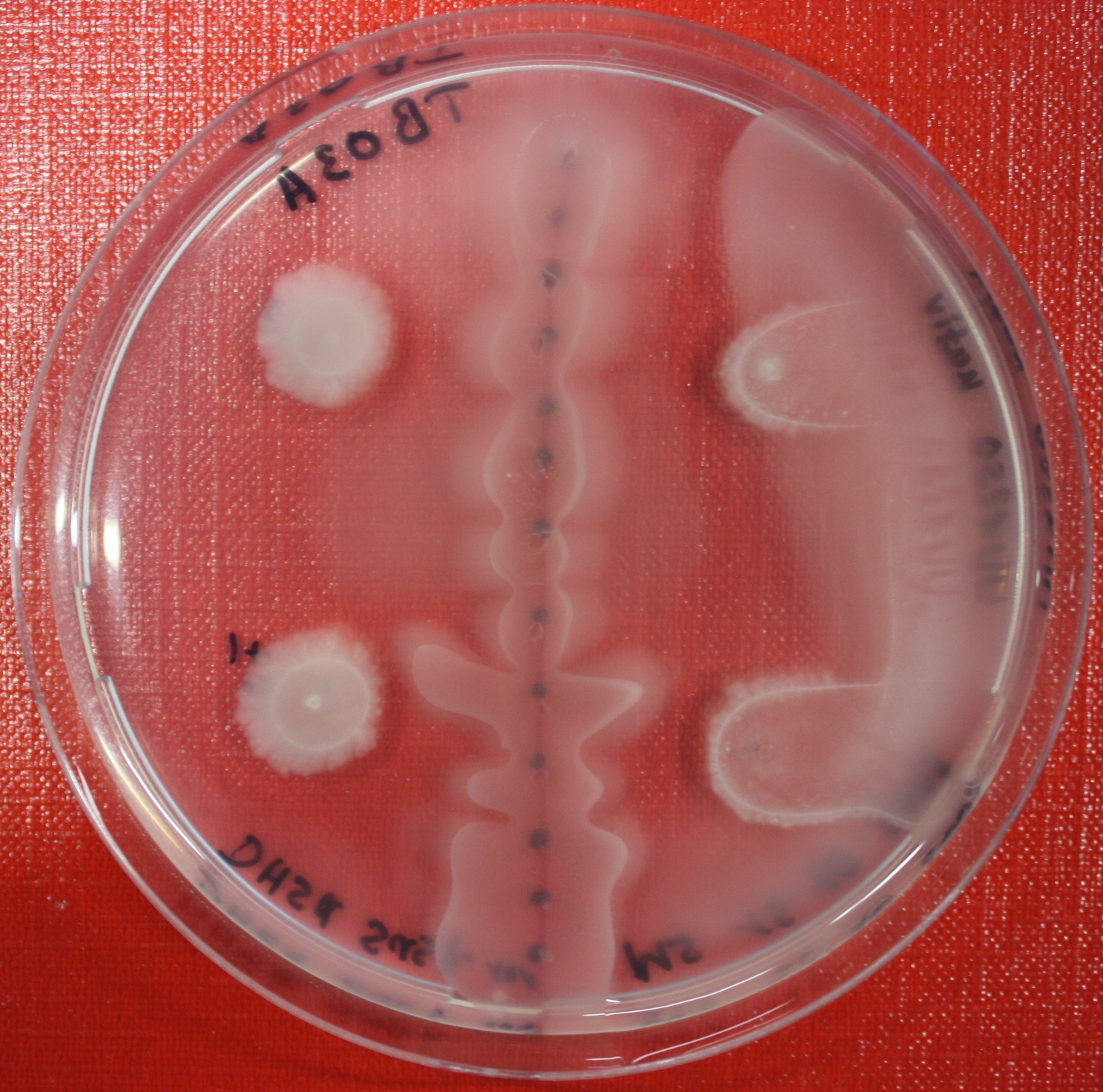
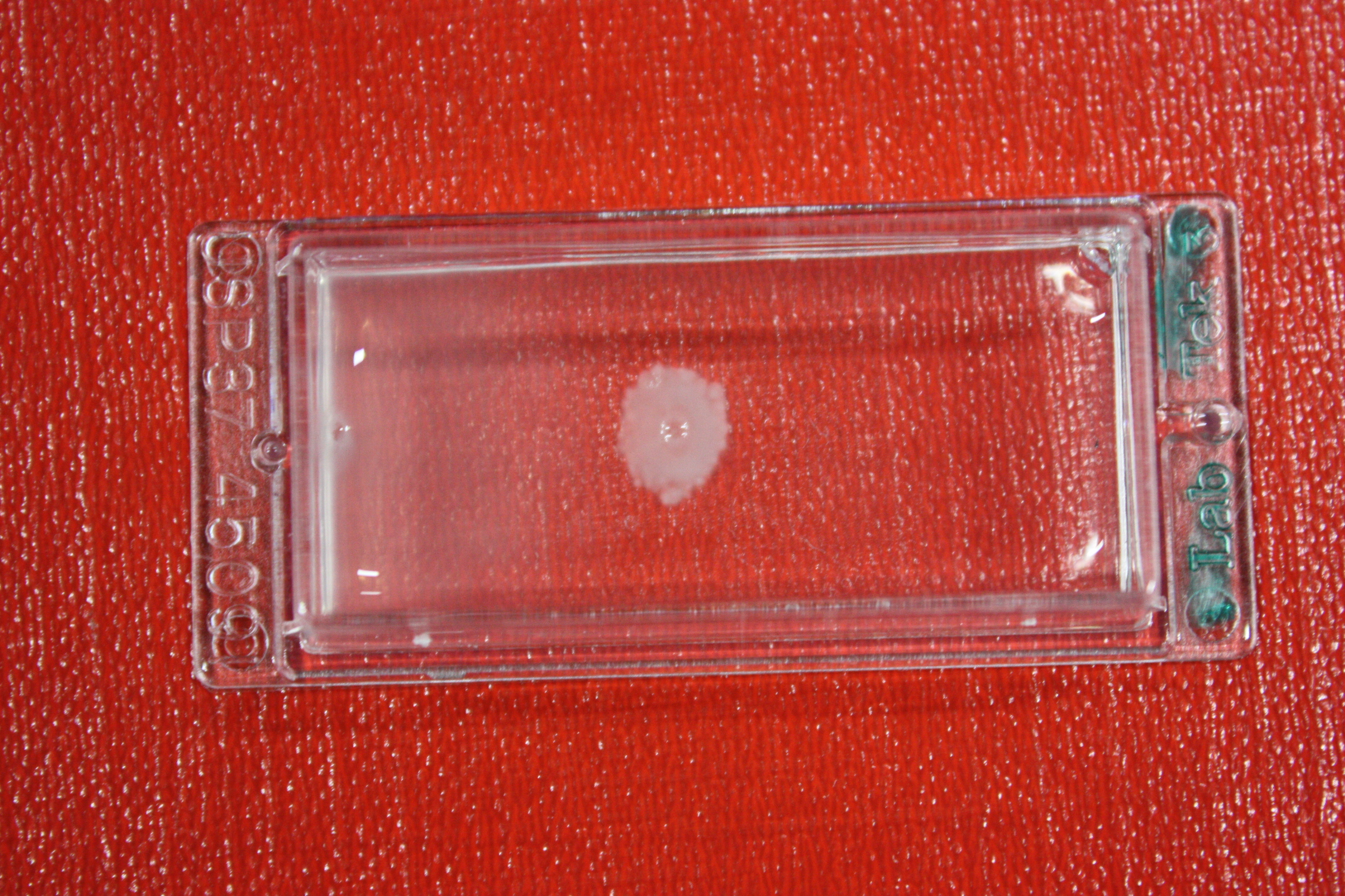
[[Image:SwarmA_CA_line.jpg|left|thumb|400px|Center attractant plug line]][[Image:SwarmA_CA_spot.jpg|right|thumb|400px|Spotted attractants]] | [[Image:SwarmA_CA_line.jpg|left|thumb|400px|Center attractant plug line]][[Image:SwarmA_CA_spot.jpg|right|thumb|400px|Spotted attractants]] | ||
| - | [[Image:SwarmA_fluid_attractant.jpg|left|thumb|400px|Center fluid attractant line]] [[Image:SwarmA_alternative_chamber.jpg|left|thumb|400px|This picture is showing an alternative chamber]] | + | [[Image:SwarmA_fluid_attractant.jpg|left|thumb|400px|Center fluid attractant line]] [[Image:SwarmA_alternative_chamber.jpg|left|thumb|400px|This picture is showing an alternative chamber. The attractant was spotted on the left side of the chamber.]] |
<br><br><br><br><br><br><br><br><br><br><br><br><br><br><br><br><br><br><br><br><br><br><br><br><br><br><br><br><br><br><br><br><br><br><br><br><br><br><br><br><br> | <br><br><br><br><br><br><br><br><br><br><br><br><br><br><br><br><br><br><br><br><br><br><br><br><br><br><br><br><br><br><br><br><br><br><br><br><br><br><br><br><br> | ||
| - | + | [https://2008.igem.org/Team:Heidelberg/Notebook/Visualization/Methods back up]<br><br> | |
| - | + | [https://2008.igem.org/Team:Heidelberg/Notebook/visualization '''back to the visualization notebook'''] | |
Latest revision as of 19:38, 29 October 2008


Visualization - Methods revealed
back to the visualization notebook
Contents |
Microscopy
Was performed using LabtekTM chambers (Nunc, Rochester, NY, USA) in two formats:
Samples were monitored using an Applied Precision - DeltaVision wide field microscope. After the first experiments have been done in bright-field mode, further experiments were only performed with fluorescent strains. They are much more accurate and are much more suitable for quantitative analysis methods.
Frames
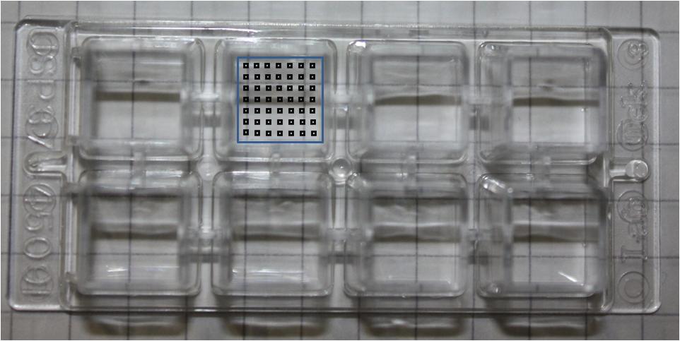
To analyse chamber samples at several time points (e.g. after 3,6,9 hours ...)
under the microscope a regular pattern for image acquisition was needed. Therefore several frames have been developed, which cover the chamber as good as possible and give the best insights into the events of the experiment.
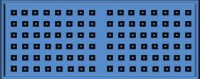
On the right side is one example for each type of chamber:
Every black spot stands for a taken picture at this position.
The rectangles are just examples of potential frames.
For small chambers square frames were used like 10x10 or 8x8, resulting in 100 or 64 pictures in total. To cover the complete area of a large chamber two separate frames had to be used. Each of those frames contained 6x8 (6 in height and 8 in width) images.
chemotactical activity
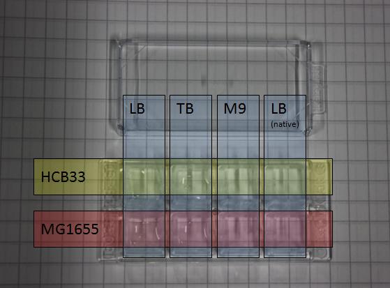
This test series was used to test the chemotactic activity of strains depending on special strain abilities and the media they were incubated in or transferred to.
3 µl of an overnight culture were put into a small chamber filled with 200 µl of the appropriate media.
The activity of the bacteria has been observed over several hours. Depending on the experiment sometimes after a specific time an attractant like casamino acids has been added to the media to test the effect of the attractant on the activity of the specific strain.
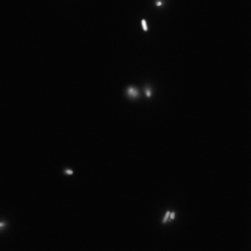
This was performed with short time lapse series like taking 90 pictures at one position with a time lapse of less than 0.33 seconds.
This experiment may give an idea of the behavior of certain strains under specific conditions.
With this information it is easier to choose the right strain and the best conditions for further experiments.
It is also possible to predict the bacterial behavior, so that some parameters can be excluded, if the bacteria do not act as expected.
Here is one example of such a time lapse serie:
To see this video the quicktime plugin for the appropriate browser is needed. The [http://www.apple.com/de/quicktime/download/ Quicktime] player is freely available and can be downloaded from apple.com
computer-assisted analysis
ImageJ
The Deltavision wide field microscope creates Deltavision files (.dv) as output, which may be in stacks or not colored as wanted. To automatically convert the vast amount of generated .dv files into Jpeg files and to process the images, homemade plugins for ImageJ were used. (For example by coloring and/or merging.)
For the automatic processing an importer plugin [http://www.loci.wisc.edu/ome/formats-imagej.html LOCI Bio-Formats] was used. The link can be found by clicking on the name.
This plugin enables the automatic processing of Deltavision files into ImageJ.
An example for such a plugin would be:
Just click on the picture above to see the plugin.
The plugin *.txt has to be in the macros folder which is located in the ImageJ mainfolder, then the plugin can be run from windows with the following command in the commandline:
java -jar ij.jar -batch nameoftheplugin
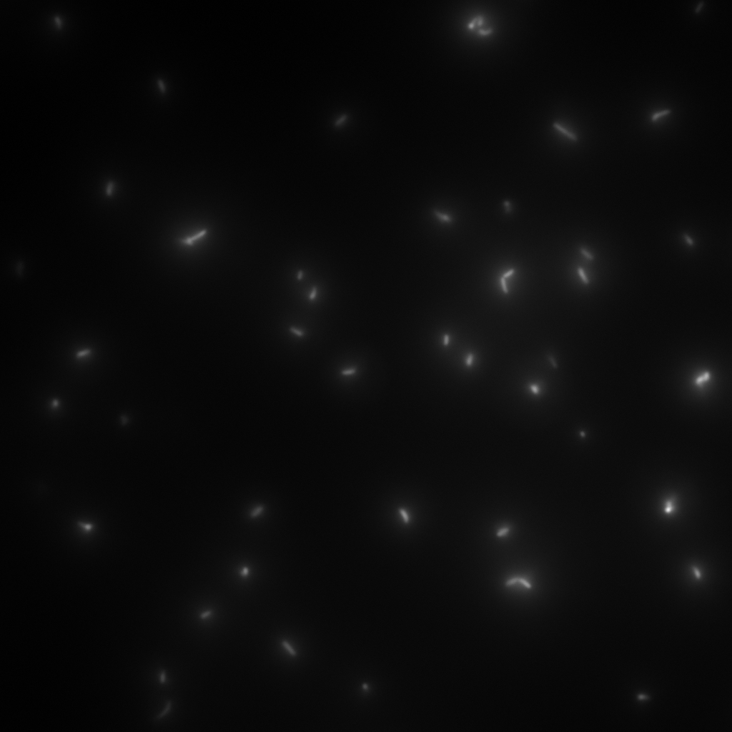
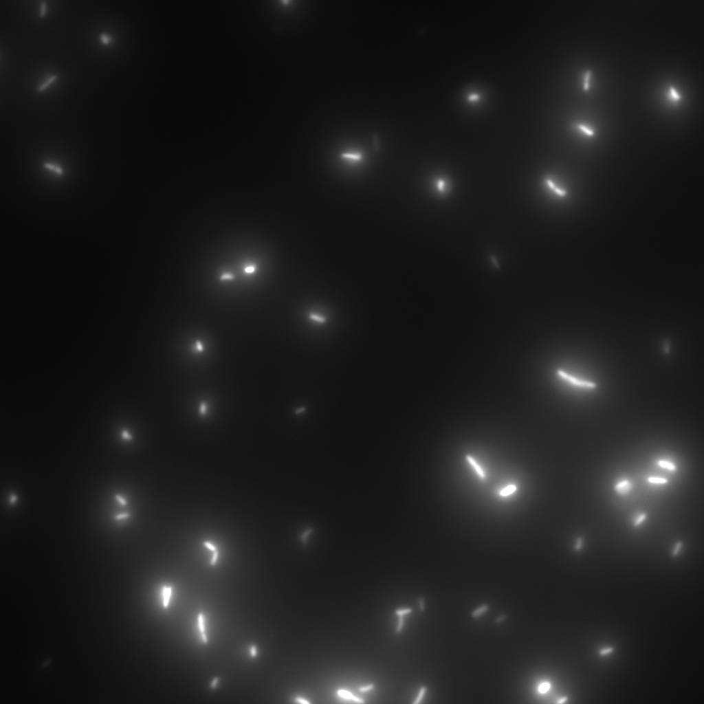
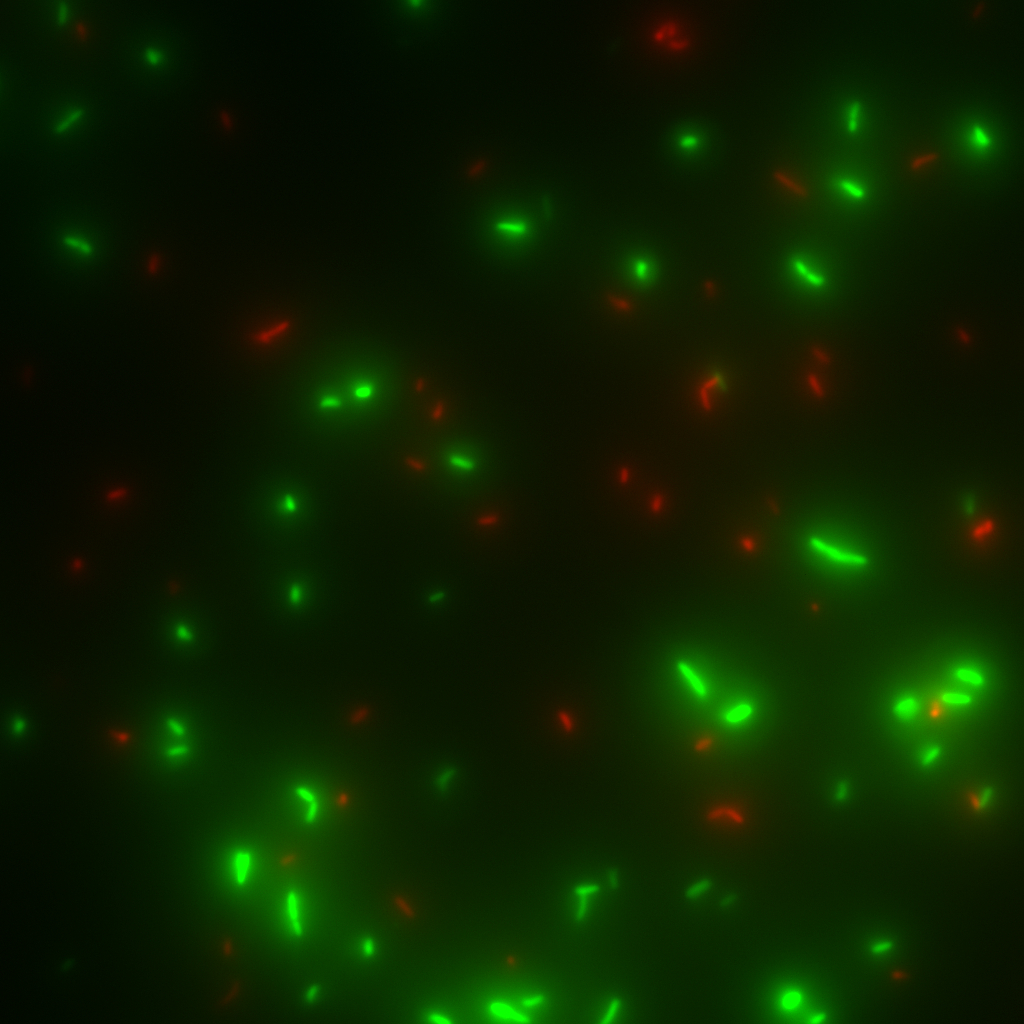
This plugin takes a serie of 64 pictures taken with the Deltavision microscope in the specific folder.
Each file was a stack of 2 pictures with two different channels. The plugin opens the files merges them to one RGB picture, converts them to Jpeg and saves the new pictures in the same folder.
Those grey pictures are 2 pictures forming one stack, the third one is the product of the plugin:
Analysis with MatLab
Furthermore every picture can be correlated with an intensity value.
In combination with an automatic picture arrangement function, which many image processing programs provide, it is possible to create 3D graphics, which can be compared with their frame pictures.
To see some results of this image processing and analysis: ~~click here~~
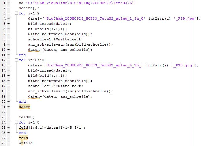
An example of analysing the left frame of an experiment with the large chamber:
Just click on the picture above to see the code.
There are several other possibilities to change the calculation of the parameters and adjust the 3D graphic.
This can be combined with analysing the right frame as well.
If the result like here would be A=feld and if the result of the right frame is B=feld both frames can be combined and shown as a 3D grapic with the following commands:
C=[A,B]
surf(C')
shading interp
Examples of this can be seen on the click here link above.
back up
Swarm Assays
PROTOCOL FOR SWARM-PLATE CHEMOTAXIS AGAINST A POSSIBLE ATTRACTANT:
This protocol was created using petri-dishes. But every other chamber could be used as well.
- Step 1: Make sure you have everything ready to get started. You need:
- Petri-dishes. !!! sign your petri-dishes before You pour in the media. Also mark the spots where you want to set the attractant or attractant line and the bacteria. !!! Handle the soft agar with care. After the addition of the attractant the petri-dish should only be moved really carefully.
- 50 ml falcons
- 25 ml media containig 0.2%-0.3% Agar for every petri-dish.
- samples of the appropriate attractants. The concentration depends on several substance depending attributes.
- Other substances like antibiotics (Amp, Kan, Cm) or inducer (IPTG, Arabinose)
- Step 2: Your agar-media solution should be clear and the agar completely dissolved. If you want to use attractant plugs1 or other non fluid attractants, go first through step 5 then back through 2,3,4 skip 5, further with 6 and so on...
- Step 3: Take Take a 50 ml falcon pour 25 ml of your agar containing media in it and add antibiotics or inducing substances. If no extra substances are needed just skip this step.
- Step 4: Let your media polimerize. At least let it rest for 15/20 min.
- Step 5: Then add the attractant. e.g.: a casamino acid solution
- Step 6:
- Put the whole plate into a 4°C fridge for 12-16 hours to allow the attractant to build up a gradient.
- Make an overnight culture of the strains you want to test, use TB media and add inducing substances if something has to be induced.
Next day:
- Step 7: Take your overnight culture. It should be at an OD of 0.4-0.6. Then take 1 ml of the bacteria suspension and centrifuge it for 10 minutes at 4,000 rpm. Resolve the pellet at 100 µl of the media you are using in the petri-dish.
- Step 8: Place 3-6 µl of your purrified bacteria at the premarked spots on the petri-dish sample.
- Step 9: Put the whole plate into the incubator at ~30°C and take a look at your plates after 24, 48 and 72 hours. Put the plates into a plastic bag like the small ones for the bench trash to protect the plates from running dry to fast. Only move the plates if necessary.
1: Attractant plugs can be created by adding agar to the attractant solution.
back up
back to the visualization notebook
 "
"
