From 2008.igem.org

(Difference between revisions)

Latest revision as of 00:42, 30 October 2008

Model Construction

Other pages:

Introduction

This approach is mainly based on a bibliographical work. We found essential to choose only parameters that could be found in literature so as to get quickly a first idea of the way our system could behave.
In this section, we will present the model we chose to describe the evolution of our system's concentrations.

Classical model and temporal rescaling

Classically we use the following equation to model gene interactions (see for example in [1]) :

where [Y] denotes the concentration of Y protein and γ its degradation rate (which unit is time^-1).

This system has been extensively studied in S.Kalir and U. Alon article. A lot of experimental data obtained in similar experimental conditions are available. Moreover models have been built for the FIFO part of the system so that we were able to use directly their experimentally determined parameters. When we did not find relevant information, we chose a classical Hill function.

To decrease the number of parameters we normalized every protein concentration, so that their value would range between 0 and 1. Moreover, we found it convenient because it enabled us to compare the respective influences of these concentrations.

Furthermore, it is important to note that this degradation rate represents both the influence of the degradation and dilution. We assume that the degradation can be neglected compared to the dilution caused by the cell growth. Thus, every degradation rates are assumed equal. We kept the designation “degradation rate” for convenience, so as not to mix up with the dilution that might occur elsewhere.

We therefore wanted to have a proper time scale. By setting the degradation rates, γ ,to 1, a time unit corresponds to . Since we can know easily the value of the real half-time, we may know the real timescale out of our computations. Then we have:

Finally, the key problem with a dynamic system consists in the fact that adding a new equation gives a more detailed idea of the overall process, but one looses meaning by doing so since new undefined parameters appear. Hence, it becomes hard to link those parameters with a biological meaning and reality. In that respect, we chose not to introduce the mRNA state between transcription and translation in our model. We presented things as if a protein would act directly upon the following.

Conclusion

We finally obtained the following equations :

and the following parameters :

Parameter Table
Parameter	Meaning	Original Value	Normalized Value	Unit	Source
γ	Degradation rate	0.0198	1	min^-1	wet-lab
β_FliA	FlhDC activation coefficient	50	0.1429	min^-1	[1]
β'_FliA	FliA activation coefficient	300	0.8571	min^-1	[1]
β_CFP	FlhDC activation coefficient	1200	0.8276	min^-1	[1]
β'_CFP	FliA activation coefficient	250	0.1724	min^-1	[1]
β_YFP	FlhDC activation coefficient	150	0.3333	min^-1	[1]
β'_YFP	FliA activation coefficient	300	0.6667	min^-1	[1]
β_EnvZ-RFP	FlhDC activation coefficient	100	0.2222	min^-1	[1]
β'_EnvZ-RFP	FliA activation coefficient	350	0.7778	min^-1	[1]
β_FlhDC	Maximum production rate		1	min^-1	∅
n_envZ	Hill coefficient		4	¤	∅
θ_envZ	Hill characteristic concentration		0.5	c.u	∅

Now you have had a good overlook of our model, go see a more detailed justification where our normalization choices are thouroughly explained :

↓ Detailed justification ↑

We shall present here a more detailed presentation of the choice we made as far as our model is concerned

Sum effect and linear modelling

The flagella gene network has been thoroughly studied in [1]. We used two major results presented in this study. Firstly, Shiraz Kalir and Uri Alon came up with the fact that the promoters of class 2 genes, among which fliL, flgA and flhB, behaved like SUM-gate functions with flhDC and fliA inputs. Secondly, their experiments proved that these influences could be considered as linear. Thus the following model:

β and β’ represent the relative influence of flhDC and fliA respectively, the units of β and β’ being time^-1.

Furthermore, they came up with numerical values of β and β’ for each gene, which fitted quite well to their experiments. Since our experimental conditions are similar to those described in the article, we decided that we could use those values as well in our model.
Thus the resulting equations

Hill function

When we had no relevant information, we decided to model the promoter activity by a Hill function. This was the case for the effect of envZ over FlhDC :

Thus the dynamic equation for [FlhDC] :

As for the parameters, we decided to chose biologically feasible values, that is n_EnvZ=4 and θ_EnvZ=0.5.

Normalization

FliA, CFP, YFP, EnvZ-RFP

We kept the β and β’ values found by S. Kalir and U. Alon, since they showed the relative influence of flhDC and fliA. To have the same order of magnitude between each specie, we normalized those parameters between 0 and 1 as following. We reasoned independently for each equation, wishing to set the equilibrium values of the concentration to 1 given input values of 1. With the values taken from S. Kalir and U. Alon, this gave:

In fact, if we take CFP for example:

The maximum of [CFP] is reached when [fliA] = 1 and [flhDC] = 1 ; when we solve with these condidtions, we obtain :

Then setting the equilibrium value of [CFP] to 1 corresponds to setting

The analysis of fliA is different, but not the result:

With an input of flhDC equal to 1, the solution of the differential equation is:

And the condition on the equilibrium imposes

To conclude, we see that we always get the same condition:

Finally, since we had imposed γ=1 we resulted with β+β'=1.

FlhDC

Likewise the previous analysis, we set γ_FlhDC to 1. Then, since FlhDC is fully expressed when envZ is not, we see that when solving under this conditions, we get

hence the need to set

This is highly interesting since normalization implies that β_FlhDC=1 , so that we do not need to find a value for β_FlhDC.
Furthermore, since [EnvZ] has been normalized, we have to do so for θ_EnvZ as well, since its role is to stand as a reference concentration for EnvZ. Therefore, we have to normalize it in the same way we did for [EnvZ]:

we had

which means we have to impose :

Time rescaling

We evaluated in the wet lab the half life time for our cells, and then calculated the degradation constants using :

The value for half-life time we found and used is 35min. Setting γ to one, gave us the time rescaling factor (0.0198).

Parameters table

Parameter Table
Parameter	Meaning	Original Value	Normalized Value	Unit	Source
γ	Degradation rate	0.0198	1	min^-1	wet-lab
β_FliA	FlhDC activation coefficient	50	0.1429	min^-1	[1]
β'_FliA	FliA activation coefficient	300	0.8571	min^-1	[1]
β_CFP	FlhDC activation coefficient	1200	0.8276	min^-1	[1]
β'_CFP	FliA activation coefficient	250	0.1724	min^-1	[1]
β_YFP	FlhDC activation coefficient	150	0.3333	min^-1	[1]
β'_YFP	FliA activation coefficient	300	0.6667	min^-1	[1]
β_EnvZ-RFP	FlhDC activation coefficient	100	0.2222	min^-1	[1]
β'_EnvZ-RFP	FliA activation coefficient	350	0.7778	min^-1	[1]
β_FlhDC	Maximum production rate		1	min^-1	∅
n_envZ	Hill coefficient		4	¤	∅
θ_envZ	Hill characteristic concentration		0.5	c.u	∅

c.u. being an arbitrary concentration unit.

Moreover, in order to take into account the fact that data are obtained form 'real' experiments (number of parameters, length of data set) we hereby propose a criteria to legitimate the chosen model depending on the experimental conditions, in comparison with a more general model (Hill functions).

↓ Akaike Criteria ↑

Using mathematical criteria to discriminate between model

When building a model, it is of the utmost importance to present a justification of the choice made along the transposition process from biological reality to mathematical representation. The aim of this section is to introduce a mathematical justification of the choice we made since it seems remote from biological reality. The criterion presented below are to help choosing the most relevant model given the experimental constraints.

Short introduction to the criteria

Using linear equations in a biological system might seem awkward. However, we did prove the relevance of this approach. We have been looking for a criterion that would penalize a system that had many parameters, but that would also penalize a system which quadratic error would be too important while fitting experimental values. The goal here is to decide whether, assuming that the experimental data looks like a model based on Hill functions, the linear part of the model is obsolete or not.
Several criteria taken from the information theory met our demands quite well :

Akaike criterion :

Hurvich and Tsai criterion :

Schwarz criterion :

where n denotes the number of experimental values, k the number of parameters and RSS the residual sum of squares. The best fitting model is the one for which those criteria are minimized.

It is remarkable that Akaike criterion and Hurvich and Tsai criterion are alike. AICc is therefore used for small sample size, but converges to AIC as n gets large. Since we will work with 20 points for each experiment, it seemed relevant to present both criteria. In addition, Schwarz criterion is meant to be more penalizing.

Experiment

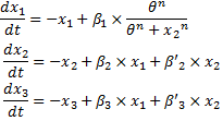
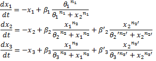
As an experiment, we compared the two models presented below :

System#1 : using the linear equations found in bibliography :

System#2 : using classical Hill functions :

We made a set of data out of a noised Hill function. In fact, our data set was made by using the same equations as System#2, but we introduced a normal noise for each point. Thus, System#1 is penalized because its RSS will be greater than that of System#2. Nevertheless, System#2 will be more penalized by its number of parameters.
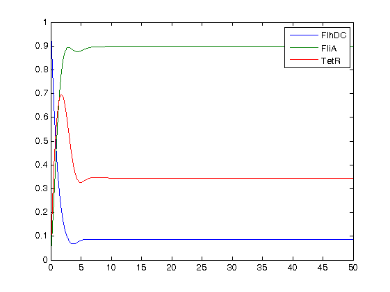
With Matlab, we run a fitting simulation for each system, and we obtained the RSS. We then evaluated the different criteria for both models. We chose to act as if the length of our experimental data set was 20 (which is what we would have gotten in reality). The results are presented below.

Comparison of the systems for n=20
Criteria	System#1	System#2
AIC	26.7654	32.0035
AICc	38.7654	168.0035
BIC	22.9435	24.3596

Comparison of the systems for n=100
Criteria	System#1	System#2
AIC	169.5495	32.1150
AICc	171.1147	38.5912
BIC	172.0100	37.0360

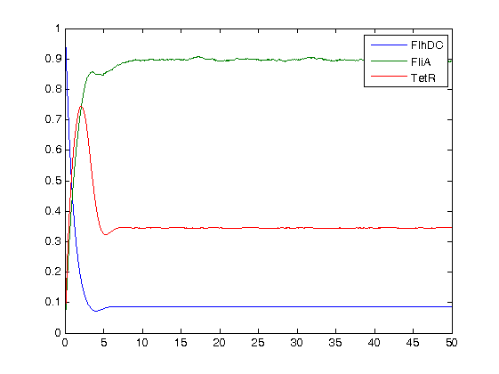
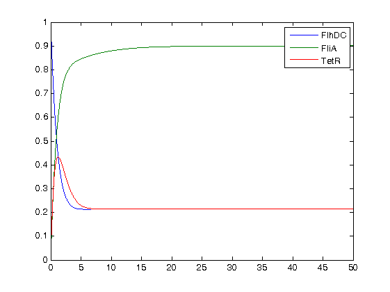
Finally, we ran the simulation plots obtained for the parameters that best fitted. Here are the results proving that no numerical errors were to be seen :

Bob Model

Hill Model

Then, we see that the model that uses linear equations does not fit that well, but under certain conditions it is not so bad. Indeed, if the data set is short, this kind model is a relevant model since it eases the understanding of the dynamics.

Consequently, what have we proved? These results show that:
- We may see that, as predicted, System#2 is not penalized anymore for greater values of n, although System#1 is. Consequently, we may adapt our system knowing the length of the data set we are going to obtain experimentally.
- However, since for a larger set of data System#2 minimizes the criteria, these criteria cannot decide whether a model is "better" than another one, since those criteria are arbitrary. Yet, they may help us find a better compromise between simplification and accuracy.
- Consequently, these criteria corroborate our choice of a linear model.

A fundamental tool?

Why can we introduce this seemingly awkward criteria as being a fundamental tool? This precise criteria enables the mathematician to adapt its model. In fact, in that respect, conducting this analysis over his model gives tangible arguments to the mathematician to use such and such model. Indeed, in our precise case, if we have about 20 experimental points to fit, the linear approach is sufficient. However, if we get 50 points, it becomes inadequate compared to a model with Hill functions. We believe that this kind of criteria is an essential tool, that might help the model maker to comprehend and control the assumptions he made while creating his model.

We mostly used the definition of the criteria given in :

[http://www.liebertonline.com/doi/pdf/10.1089/rej.2006.9.324 K. Kikkawa.Statistical issue of regression analysis on development of an age predictive equation. Rejuvenation research, Volume 9, n°2, 2006.]

Bibliography

[1] Shiraz Kalir, Uri Alon. Using quantitative blueprint to reprogram the dynamics of the flagella network. Cell, June 11, 2004, Vol.117, 713-720.

@@ Line 1: / Line 1: @@
 {{Paris/Menu}}
-<br>
+{{Paris/Header|Model Construction}}
-<center><html><div style="color:#275D96; font-size:2em;">Model construction</div></html></center>
+{{Paris/Section_contents_analysis}}
-<br>
 = Introduction =
-* This preliminary approach is mainly based on a bibliographical work. In fact, it is important to understand that with this approach, we did not intend to design the most accurate model possible. We found essential to choose only parameters that could be found in literature. The main goal was to get quickly a first idea of the way our system could behave.
+* This approach is mainly based on a bibliographical work. We found essential to choose only parameters that could be found in literature so as to get quickly a first idea of the way our system could behave.
 * In this section, we will present the model we chose to describe the evolution of our system's concentrations.
@@ Line 16: / Line 15: @@
 where [Y] denotes the concentration of Y protein and γ its degradation rate (which unit is time<sup>-1</sup>).
 <br>
-* We did a lot of bibliography work and found many interesting expressions found in [[Team:Paris/Modeling/BOB#Bibliography|S.Kalir and U. Alon article]]. We also kept the parameters values. When we did not find relevant information, we chose a classical Hill function.
+* This system has been extensively studied in [[Team:Paris/Modeling/BOB#Bibliography|S.Kalir and U. Alon article]]. A lot of experimental data obtained in similar experimental conditions are available. Moreover models have been built for the FIFO part of the system so that '''we were able to use directly their experimentally determined parameters'''. When we did not find relevant information, we chose a classical Hill function.
-* We normalized every concentration, so that their value would range between 0 and 1. Indeed, we found it necessary because we needed to be able to compare the respective influences of these concentrations.
+* To decrease the number of parameters we normalized every protein concentration, so that their value would range between 0 and 1. Moreover, we found it convenient because it enabled us to compare the respective influences of these concentrations.
-* Furthermore, it is important to note that this degradation rate represents both the influence of the degradation and dilution. We assume that the degradation can be neglected compared to the dilution caused by the cell growth. Thus, every degradation rates are equal. We kept the designation “degradation rate” for convenience, so as not to mix up with the dilution that might occur elsewhere.
+* Furthermore, it is important to note that this degradation rate represents both the influence of the degradation and dilution. We assume that the degradation can be neglected compared to the dilution caused by the cell growth. Thus, '''every degradation rates are assumed equal'''. We kept the designation “degradation rate” for convenience, so as not to mix up with the dilution that might occur elsewhere.
-* We therefore wanted to have a proper time scale. We then set the degradation rates, γ ,to 1. Since we can know easily the value of the real half-time, we may know the real timescale out of our computations. Then we have:
+* We therefore wanted to have a proper time scale. By setting the degradation rates, γ ,to 1, a time unit corresponds to . Since we can know easily the value of the real half-time, we may know the real timescale out of our computations. Then we have:
 <br>
 [[Image:Gamma_Expression.jpg|center]]
 <br>
 * Finally, the key problem with a dynamic system consists in the fact that adding a new equation gives a more detailed idea of the overall process, but one looses meaning by doing so since new undefined parameters appear. Hence, it becomes hard to link those parameters with a biological meaning and reality. In that respect, we chose not to introduce the mRNA state between transcription and translation in our model. We presented things as if a protein would act directly upon the following.
 = Conclusion =
 We finally obtained the following equations :
-[[Image:eqn_flhDC.jpg|center]]
 [[Image:FliA_dynamics.jpg|center]]
 [[Image:CFP.jpg|center]]
 [[Image:YFP.jpg|center]]
 [[Image:eqn_EnvZ-RFP.jpg|center]]
+[[Image:eqn_flhDC.jpg|center]]
 and the following parameters :
@@ Line 139: / Line 139: @@
 |}</center>
-Now you have had a good overlook of our model, go see a more [[Team:Paris/Network_analysis_and_design/Core_system/Model_construction/Detailed_justification|detailed justification]], where our normalization choices are thouroughly explained!
+Now you have had a good overlook of our model, go see a more detailed justification where our normalization choices are thouroughly explained :
+{{Paris/Toggle|Detailed justification|Team:Paris/Network_analysis_and_design/Core_system/Model_construction/Detailed_justification}}
-= Navigator =
+Moreover, in order to take into account the fact that data are obtained form 'real' experiments (number of parameters, length of data set) we hereby propose a '''criteria to legitimate the chosen model depending on the experimental conditions''', in comparison with a more general model (Hill functions).
-<center>[[Team:Paris/Network_analysis_and_design/Core_system|Back to the overall presentation of our system and model]]</center>
+{{Paris/Toggle|Akaike Criteria|Team:Paris/Network_analysis_and_design/Core_system/Model_construction/Akaike}}
-<center>[[Team:Paris/Network_analysis_and_design/Core_system/Model_construction#Introduction|Top of the page]]</center>
-<center>[[Team:Paris/Network_analysis_and_design/Core_system/Model_construction/Detailed_justification|Have a look at our detailed justification!]] [[Team:Paris/Network_analysis_and_design/Core_system/Model_construction/Akaike|Have a look at our Akaike criteria!]]</center>
+{{Paris/Navig|Team:Paris/Analysis}}
 = Bibliography =
 * [1] Shiraz Kalir, Uri Alon. ''Using quantitative blueprint to reprogram the dynamics of the flagella network.'' Cell, June 11, 2004, Vol.117, 713-720.

Team:Paris/Analysis/Construction