Team:iHKU/modelling
From 2008.igem.org
| (5 intermediate revisions not shown) | |||
| Line 235: | Line 235: | ||
<h2 class="style31"><a name="top" id="top"></a><span class="style24">CONTENTS:</span></h2> | <h2 class="style31"><a name="top" id="top"></a><span class="style24">CONTENTS:</span></h2> | ||
<ul class="style24"> | <ul class="style24"> | ||
| - | <li class="style20" | + | <li class="style20"><a href="#1">Cell Movement in Microscopic and Macroscopic Aspects</a></li> |
| - | <li class="style20" | + | <li class="style20"><a href="#2">Front propagation for Cell Growth </a></li> |
| - | <li class="style20" | + | <li class="style20"><a href="#3">Density Dependent Motility</a></li> |
| - | <li class="style20" | + | <li class="style20"><a href="#4">Full Model of Density Dependent Motility</a></li> |
| - | <li class="style20" | + | <li class="style20"><a href="#5">Results</a></li> |
</ul> | </ul> | ||
<p> </p> | <p> </p> | ||
| Line 253: | Line 253: | ||
</div> | </div> | ||
<p class="style26">Firstly, for the one dimension of random walk, let <em>x</em> (<em>t</em>) denote the position of an <em>E.coli</em> cell at time t, given that its position coincided with the point <em>x</em>=0 at time <em>t</em>=0. And we assumed an <em>E.coli</em> cell moves an average distance <em>l</em>—in either the positive or negative direction of the <em>x</em>-axis—each step (during a time (<em>τ</em>) between two tumbling states). The probability that the cell was found at the point <em>x</em> at time <em>t </em>was now equal to the probability that, in a series of <em>n</em> (=<em>t</em>/<em>τ</em>) successive moving steps, the cell made m more steps in the positive direction of the axis than in the negative direction. The desired probability was given by the binomial expression [<a href="#ref">1, 2</a>]</p> | <p class="style26">Firstly, for the one dimension of random walk, let <em>x</em> (<em>t</em>) denote the position of an <em>E.coli</em> cell at time t, given that its position coincided with the point <em>x</em>=0 at time <em>t</em>=0. And we assumed an <em>E.coli</em> cell moves an average distance <em>l</em>—in either the positive or negative direction of the <em>x</em>-axis—each step (during a time (<em>τ</em>) between two tumbling states). The probability that the cell was found at the point <em>x</em> at time <em>t </em>was now equal to the probability that, in a series of <em>n</em> (=<em>t</em>/<em>τ</em>) successive moving steps, the cell made m more steps in the positive direction of the axis than in the negative direction. The desired probability was given by the binomial expression [<a href="#ref">1, 2</a>]</p> | ||
| - | <p align="center"><img src="/wiki/images/d/de/Modelling_pic3.png" width=" | + | <p align="center"><img src="/wiki/images/d/de/Modelling_pic3.png" width="550" height="280" /></p> |
<p class="style26">where</p> | <p class="style26">where</p> | ||
| - | <p align="center" class="style26"><img src=" | + | <p align="center" class="style26"><img src="/wiki/images/7/76/Modelling_pic4.JPG" width="180" height="52" /> , </p> |
<p class="style26"><em>v</em>=<em> l</em>/<em>τ</em> was the average speed of the cell movement, and <em>f</em>=1/<em>τ </em>was the tumbling frequency of <em>E.coli</em>. </p> | <p class="style26"><em>v</em>=<em> l</em>/<em>τ</em> was the average speed of the cell movement, and <em>f</em>=1/<em>τ </em>was the tumbling frequency of <em>E.coli</em>. </p> | ||
<p class="style26">In two dimensions, the square of the distance from the origin to the point (x, y) was <em>r</em>2=<em>x</em>2+<em>y</em>2; therefore</p> | <p class="style26">In two dimensions, the square of the distance from the origin to the point (x, y) was <em>r</em>2=<em>x</em>2+<em>y</em>2; therefore</p> | ||
| - | <p align="center" class="style26"><img src=" | + | <p align="center" class="style26"><img src="/wiki/images/2/2e/Modelling_pic5.JPG" width="108" height="45" /></p> |
<p class="style26">For a macroscopic view, <em>D</em> was defined as the diffusion coefficient. Normally, as the swimming speed of <em>E.coli</em> is about 20<em>um</em>/<em>s</em> and the tumbling frequency is about 1 <em>Hz</em>, the diffusion coefficient is about 200<em>um</em>2/<em>s </em>[<a href="#ref">3</a>].</p> | <p class="style26">For a macroscopic view, <em>D</em> was defined as the diffusion coefficient. Normally, as the swimming speed of <em>E.coli</em> is about 20<em>um</em>/<em>s</em> and the tumbling frequency is about 1 <em>Hz</em>, the diffusion coefficient is about 200<em>um</em>2/<em>s </em>[<a href="#ref">3</a>].</p> | ||
| - | <p><a href="#top">[Back to Top]</a></p> | + | <p align="right"><a href="#top">[Back to Top]</a></p> |
<p> </p> | <p> </p> | ||
<h3><span class="style7"><strong><a name="2" id="2"></a>Front propagation for cell growth</strong></span> <br /> | <h3><span class="style7"><strong><a name="2" id="2"></a>Front propagation for cell growth</strong></span> <br /> | ||
</h3> | </h3> | ||
<p class="style26">If we only considered the diffusion effect and growth effect of the cell culture, it came up with the model Fisher-Kolmogorov equation which was firstly developed by R. A. Fisher and A. N. Kolmogorov [<a href="#ref">4</a>]. </p> | <p class="style26">If we only considered the diffusion effect and growth effect of the cell culture, it came up with the model Fisher-Kolmogorov equation which was firstly developed by R. A. Fisher and A. N. Kolmogorov [<a href="#ref">4</a>]. </p> | ||
| - | <div align="center" class="style26"><img src=" | + | <div align="center" class="style26"><img src="/wiki/images/8/8d/Modelling_pic6.JPG" width="387" height="41" /> </div> |
<p class="style26">where <em>ρ </em>was the cell density, <em>D</em> was the diffusion coefficient, <em>γ</em>0 was growth rate, <em>ρ</em>s was saturation density. </p> | <p class="style26">where <em>ρ </em>was the cell density, <em>D</em> was the diffusion coefficient, <em>γ</em>0 was growth rate, <em>ρ</em>s was saturation density. </p> | ||
<p class="style26">Here, due to the symmetry, we investigated equation (4) in case of cylindrical domains with u depending only on radius. Numerical study with an initially condition of Gaussian function as Fig.2 can give a solution shown in Fig.2, while analytical solution can refer to reference [<a href="#ref">5</a>]. Based on the solution, it was found that the speed of the front propagation of the pattern was proportional to the square root of the product of diffusion coefficient <em>D</em> and growth rate <em>γ</em>. As this migration speeds of the cell pattern at different <em>cheZ</em> expression levels can be obtained from experiments, and the growth rate was also measured, the diffusion coefficient <em>D</em> at different <em>cheZ</em> expression levels were also known then. And the cell density can be transformed to the brightness that we observed in the experiments <a href="/wiki/Team:iHKU/result">(see the brightness model part)</a>, the quantity <em>ρ</em> can be compared with the experiments. Therefore, each quantity in equation (4) can be compared with the experiments. </p> | <p class="style26">Here, due to the symmetry, we investigated equation (4) in case of cylindrical domains with u depending only on radius. Numerical study with an initially condition of Gaussian function as Fig.2 can give a solution shown in Fig.2, while analytical solution can refer to reference [<a href="#ref">5</a>]. Based on the solution, it was found that the speed of the front propagation of the pattern was proportional to the square root of the product of diffusion coefficient <em>D</em> and growth rate <em>γ</em>. As this migration speeds of the cell pattern at different <em>cheZ</em> expression levels can be obtained from experiments, and the growth rate was also measured, the diffusion coefficient <em>D</em> at different <em>cheZ</em> expression levels were also known then. And the cell density can be transformed to the brightness that we observed in the experiments <a href="/wiki/Team:iHKU/result">(see the brightness model part)</a>, the quantity <em>ρ</em> can be compared with the experiments. Therefore, each quantity in equation (4) can be compared with the experiments. </p> | ||
| Line 306: | Line 306: | ||
<p>in 2D(left) and 3D(right) </p> | <p>in 2D(left) and 3D(right) </p> | ||
</div> | </div> | ||
| - | <p><a href="#top">[Back to Top]</a></p> | + | <p align="right"><a href="#top">[Back to Top]</a></p> |
<p> </p> | <p> </p> | ||
<h3 class="style3"><strong><a name="3" id="3"></a><span class="style7">Density Dependent Motility</span></strong></h3> | <h3 class="style3"><strong><a name="3" id="3"></a><span class="style7">Density Dependent Motility</span></strong></h3> | ||
| - | <p align="center"><img src=" | + | <p align="center"><img src="/wiki/images/0/0a/Modelling_pic7.JPG" alt="" width="265" height="114" /></p> |
<div align="center"><span class="style27">Fig. 3</span> Designed genetic circuit</div> | <div align="center"><span class="style27">Fig. 3</span> Designed genetic circuit</div> | ||
<p class="style26">In experiments, we designed a circuit that the cell motility was repressed by cell density <em>ρ</em>. When the cell density <em>ρ</em> was high, the diffusion coefficient <em>D</em> became small. Therefore, the fisher’s equation as equation (4) was not valid in this case any more. </p> | <p class="style26">In experiments, we designed a circuit that the cell motility was repressed by cell density <em>ρ</em>. When the cell density <em>ρ</em> was high, the diffusion coefficient <em>D</em> became small. Therefore, the fisher’s equation as equation (4) was not valid in this case any more. </p> | ||
<p class="style26">To order to be simplified, we firstly considered the one dimension problem again. We assumed the cell density at point <em>x</em> was <em>ρ</em>(x) at time <em>t</em>. In a very short time <em>τ</em>, there would be two groups of<em> cell </em>at <em>x</em> moving into its nearby points <em>x</em>-<em>δ</em>, <em>x</em>+<em>δ,</em> due to the random walk. And the amount of cell in each group were proportional to the product of <em>D</em>(<em>ρ</em>(<em>x</em>)) and <em>ρ</em>(<em>x</em>). Therefore,</p> | <p class="style26">To order to be simplified, we firstly considered the one dimension problem again. We assumed the cell density at point <em>x</em> was <em>ρ</em>(x) at time <em>t</em>. In a very short time <em>τ</em>, there would be two groups of<em> cell </em>at <em>x</em> moving into its nearby points <em>x</em>-<em>δ</em>, <em>x</em>+<em>δ,</em> due to the random walk. And the amount of cell in each group were proportional to the product of <em>D</em>(<em>ρ</em>(<em>x</em>)) and <em>ρ</em>(<em>x</em>). Therefore,</p> | ||
| - | <p align="center" class="style26"><img src=" | + | <p align="center" class="style26"><img src="/wiki/images/6/67/Modelling_pic8.JPG" width="456" height="170" /></p> |
| - | <p class="style26">And the function <em>D</em><em>ρ</em>(<em>ρ</em>) was a decrease function. For a simplest case, we considered a Heaviside Function</p> <p align="center" class="style26"><img src=" | + | <p class="style26">And the function <em>D</em><em>ρ</em>(<em>ρ</em>) was a decrease function. For a simplest case, we considered a Heaviside Function</p> <p align="center" class="style26"><img src="/wiki/images/c/c3/Modelnew1.png" width="254" height="217" /></p> |
<div align="center" class="style27">Fig. 4 Heaviside Function <span class="style26"><em>D</em><em>ρ</em>(<em>ρ</em>) </span></div> | <div align="center" class="style27">Fig. 4 Heaviside Function <span class="style26"><em>D</em><em>ρ</em>(<em>ρ</em>) </span></div> | ||
<p class="style26">The numerical simulations gave us the results shown in Fig.5. The cell density showed a periodical-narrow-peak structure. These peaks were what we wanted, as they produced some regions of low cell density, though the whole pattern was not quite similar with that of experiments. </p> | <p class="style26">The numerical simulations gave us the results shown in Fig.5. The cell density showed a periodical-narrow-peak structure. These peaks were what we wanted, as they produced some regions of low cell density, though the whole pattern was not quite similar with that of experiments. </p> | ||
| - | <p><img src=" | + | <p><img src="/wiki/images/d/dc/Modelnew2.png" width="561" height="272" /></p> |
<div align="center" class="style27"> | <div align="center" class="style27"> | ||
<p>Fig. 5 Periodical-narrow-peak pattern in 2D(left);</p> | <p>Fig. 5 Periodical-narrow-peak pattern in 2D(left);</p> | ||
| Line 325: | Line 325: | ||
<h3><a name="4" id="4"></a><span class="style7">Full Model of Density Dependent Motility</span></h3> | <h3><a name="4" id="4"></a><span class="style7">Full Model of Density Dependent Motility</span></h3> | ||
<div align="center"> | <div align="center"> | ||
| - | <p><img src=" | + | <p><img src="/wiki/images/0/01/Modelling_pic10.png" width="386" height="242" /></p> |
<span class="style27">Fig. 6</span> The entire designed genetic circuit </div> | <span class="style27">Fig. 6</span> The entire designed genetic circuit </div> | ||
<p class="style26">Actually, in our genetic circuit, we transformed a plasmid which can secrete AHL to environment (Fig.6). When the AHL density <em>h</em> of environment was high, the AHL came into the cell. Then AHL combining with <em>LuxR</em> repressed the expression level of <em>cheZ</em> which controled the motility of <em>E.coli.</em> So it was necessary to take account of the AHL effect. </p> | <p class="style26">Actually, in our genetic circuit, we transformed a plasmid which can secrete AHL to environment (Fig.6). When the AHL density <em>h</em> of environment was high, the AHL came into the cell. Then AHL combining with <em>LuxR</em> repressed the expression level of <em>cheZ</em> which controled the motility of <em>E.coli.</em> So it was necessary to take account of the AHL effect. </p> | ||
<p class="style26">First, the AHL was synthesized by the <em>E.coli</em> cell at the rate <em>λ</em>. And the degradation rate<em> β</em> of AHL whose half life is normally about 15 to 30 minutes. Considering the diffusion of AHL, we obtained </p> | <p class="style26">First, the AHL was synthesized by the <em>E.coli</em> cell at the rate <em>λ</em>. And the degradation rate<em> β</em> of AHL whose half life is normally about 15 to 30 minutes. Considering the diffusion of AHL, we obtained </p> | ||
<div align="center"> | <div align="center"> | ||
| - | <p><img src=" | + | <p><img src="/wiki/images/5/5b/Modelling_pic11.JPG" width="526" height="445" /> </p> |
<blockquote> | <blockquote> | ||
<blockquote> | <blockquote> | ||
| Line 340: | Line 340: | ||
</div> | </div> | ||
<p class="style26">For the nutrient, we made an assumption that the amount of nutrient consumed were proportional to the amount of cell increasing. Taking account of the nutrient diffusion, we had</p> | <p class="style26">For the nutrient, we made an assumption that the amount of nutrient consumed were proportional to the amount of cell increasing. Taking account of the nutrient diffusion, we had</p> | ||
| - | <div align="center"><img src=" | + | <div align="center"><img src="/wiki/images/5/58/Modelling_pic12.JPG" width="406" height="58" /> </div> |
<span class="style26">where <em>k</em> was the ratio that nutrient converts to cell mass. </span> | <span class="style26">where <em>k</em> was the ratio that nutrient converts to cell mass. </span> | ||
<p class="style26">We used several possible forms of function <em>Dρ</em>(<em>h</em>)(see <a href="#Drho">Results Section2</a>). The results showed that if the cell diffusion coefficient decreases fast near the AHL density threshold, the pattern came out as a multiple-ring one(<a href="#Drho">Results Section2 (a),(e)</a>). On the contrary, there was only one-ring pattern. </p> | <p class="style26">We used several possible forms of function <em>Dρ</em>(<em>h</em>)(see <a href="#Drho">Results Section2</a>). The results showed that if the cell diffusion coefficient decreases fast near the AHL density threshold, the pattern came out as a multiple-ring one(<a href="#Drho">Results Section2 (a),(e)</a>). On the contrary, there was only one-ring pattern. </p> | ||
<p><span class="style26">Therefore, in order to to make this curve <em>Dρ</em>(<em>h</em>) decreasing sharply near the threshold, it followed a prediction that we can get a multiple-ring pattern by making an auto-activate genetic circuit which the combination of LuxR and AHL can activate the expression level of itself</span>. </p> | <p><span class="style26">Therefore, in order to to make this curve <em>Dρ</em>(<em>h</em>) decreasing sharply near the threshold, it followed a prediction that we can get a multiple-ring pattern by making an auto-activate genetic circuit which the combination of LuxR and AHL can activate the expression level of itself</span>. </p> | ||
<div align="center"> | <div align="center"> | ||
| - | <p><img src=" | + | <p><img src="/wiki/images/f/f4/Modelling_pic13.png" width="329" height="221" /> </p> |
<span class="style27">Fig.8</span> The designed genetic circuit for predicted pattern</div> | <span class="style27">Fig.8</span> The designed genetic circuit for predicted pattern</div> | ||
| - | <p class="style26">Furthermore, we did some two-spot patterns which initially have two points of <em>E.coli</em> cell, so as to compare with the experiments culture (<a href="#result3">Results Section3</a>). </p> <p align=" | + | <p class="style26">Furthermore, we did some two-spot patterns which initially have two points of <em>E.coli</em> cell, so as to compare with the experiments culture (<a href="#result3">Results Section3</a>). </p> <p align="right"><a href="#top">[Back to Top]</a></p> |
<p align="left"> </p> | <p align="left"> </p> | ||
<h3 align="left"><strong><a name="5" id="5"></a><span class="style7">Result</span></strong><span class="style7">s</span></h3> | <h3 align="left"><strong><a name="5" id="5"></a><span class="style7">Result</span></strong><span class="style7">s</span></h3> | ||
| Line 354: | Line 354: | ||
<p class="style25">1. Cell Growth</p> | <p class="style25">1. Cell Growth</p> | ||
<p class="style26">In the cell growth term, we considered the growth rate was related to nutrient concentration. When the nutrient was consumed by the cell, the grow rate of the cell would decrease (<a href="#F7">Fig. 7</a>). There was a maximum growth rate <em>γ</em>0, when the nutrient was rich. The parameter <em>κ </em>described the sharp of this curve(<a href="#F7">Fig. 7</a>). The larger <em>κ</em> gave us more smooth increasing curve. And we made an assumption that one unit of nutrient would change to cell number with a ratio α. Also in the initial condition, the nutrient concentration ni can influence the patterns. Therefore, the effects of all the four parameters were studied in our model.</p> | <p class="style26">In the cell growth term, we considered the growth rate was related to nutrient concentration. When the nutrient was consumed by the cell, the grow rate of the cell would decrease (<a href="#F7">Fig. 7</a>). There was a maximum growth rate <em>γ</em>0, when the nutrient was rich. The parameter <em>κ </em>described the sharp of this curve(<a href="#F7">Fig. 7</a>). The larger <em>κ</em> gave us more smooth increasing curve. And we made an assumption that one unit of nutrient would change to cell number with a ratio α. Also in the initial condition, the nutrient concentration ni can influence the patterns. Therefore, the effects of all the four parameters were studied in our model.</p> | ||
| - | <p align="center" class="style26"><img src=" | + | <p align="center" class="style26"><img src="/wiki/images/a/a7/Modelnew3.png" width="541" height="441" /></p> |
<p class="style26">Above reuslts indicated that, the faster cell growth (larger <em>γ0 </em>and smaller doubling time) formed a smaller and a little more unclear ring pattern. And the inner ring diameter would become a litter more large when the growth rate increased. </p> | <p class="style26">Above reuslts indicated that, the faster cell growth (larger <em>γ0 </em>and smaller doubling time) formed a smaller and a little more unclear ring pattern. And the inner ring diameter would become a litter more large when the growth rate increased. </p> | ||
| - | <div align="center"><span class="style26"><img src=" | + | <div align="center"><span class="style26"><img src="/wiki/images/6/6d/Modelnew4.png" width="535" height="441" /></span> </div> |
<p class="style26">From above figures, it was found that the initial nutrient concentration ni had little influence to the pattern, especially when it was large. The only effect we observed was that smaller initial nutrient concentration ni made the ring slightly wider and more clear.</p> | <p class="style26">From above figures, it was found that the initial nutrient concentration ni had little influence to the pattern, especially when it was large. The only effect we observed was that smaller initial nutrient concentration ni made the ring slightly wider and more clear.</p> | ||
| - | <div align="center"><img src=" | + | <div align="center"><img src="/wiki/images/6/6c/Modelnew5.png" width="543" height="444" /> </div> |
<p class="style26">Here, the value of <em>κ </em>was related to the initial nutrient concentration ni. When initial nutrient concentration ni was fixed, a smaller <em>κ </em>parameter gave us the similar results with that of faster cell growth. </p> | <p class="style26">Here, the value of <em>κ </em>was related to the initial nutrient concentration ni. When initial nutrient concentration ni was fixed, a smaller <em>κ </em>parameter gave us the similar results with that of faster cell growth. </p> | ||
| - | <div align="center"><img src=" | + | <div align="center"><img src="/wiki/images/5/51/Modelnew6.png" width="545" height="447" /></div> |
<p>When we increased the value of <em>k</em>, the patterns did not change a lot, but only became a little more clearly.</p> | <p>When we increased the value of <em>k</em>, the patterns did not change a lot, but only became a little more clearly.</p> | ||
<p>In conclusion, the simulation results showed that the parameters of maximum growth rate <em>γ0 </em>and <em>κ</em> had a more important role on the ring-like pattern. And the other two parameters <em>k </em>and ni did not influence the pattern much. </p> | <p>In conclusion, the simulation results showed that the parameters of maximum growth rate <em>γ0 </em>and <em>κ</em> had a more important role on the ring-like pattern. And the other two parameters <em>k </em>and ni did not influence the pattern much. </p> | ||
| Line 369: | Line 369: | ||
<table width="200" border="1"> | <table width="200" border="1"> | ||
<tr> | <tr> | ||
| - | <td><div align="center"><a href="#Drho1"><img src=" | + | <td><div align="center"><a href="#Drho1"><img src="/wiki/images/e/e4/Modelnew7.JPG" width="180" height="220" /></a></div></td> |
| - | <td><a href="#Drho2"><img src=" | + | <td><a href="#Drho2"><img src="/wiki/images/6/67/Modelnew8.JPG" width="180" height="220" /></a></td> |
| - | <td><a href="#Drho3"><img src=" | + | <td><a href="#Drho3"><img src="/wiki/images/3/31/Modelnew9.JPG" width="180" height="220" /></a></td> |
</tr> | </tr> | ||
</table> | </table> | ||
<table width="573" border="1"> | <table width="573" border="1"> | ||
<tr> | <tr> | ||
| - | <td width="184" height="232" class="style26"><a href="#Drho4"><img src=" | + | <td width="184" height="232" class="style26"><a href="#Drho4"><img src="/wiki/images/9/97/Modelnew10.JPG" width="180" height="220" /></a></td> |
| - | <td width="373" class="style26"><a href="#Drho5"><img src=" | + | <td width="373" class="style26"><a href="#Drho5"><img src="https://static.igem.org/mediawiki/2008/5/5f/Modelnew11.JPG" width="180" height="220" /></a></td> |
</tr> | </tr> | ||
</table> | </table> | ||
| Line 384: | Line 384: | ||
<p class="style25"><a name="result3" id="result3"></a>3. Funny Pattern</p> | <p class="style25"><a name="result3" id="result3"></a>3. Funny Pattern</p> | ||
<p>With the initial conditions of two or more spots, we obtained the below funny patterns which are amazing similar with that of experiments<a href="/wiki/Team:iHKU/result">(results)</a>.</p> | <p>With the initial conditions of two or more spots, we obtained the below funny patterns which are amazing similar with that of experiments<a href="/wiki/Team:iHKU/result">(results)</a>.</p> | ||
| - | <p align="center"><img src=" | + | <p align="center"><img src="/wiki/images/8/85/Modelnew12.png" width="384" height="508" /></p> |
<p class="style25"><a name="ref" id="ref"></a>Reference:</p> | <p class="style25"><a name="ref" id="ref"></a>Reference:</p> | ||
<ul> | <ul> | ||
| Line 392: | Line 392: | ||
<li class="style25">[4] R. A. Fisher, Ann. Eugenics <strong>7</strong>, 353 (1937)</li> | <li class="style25">[4] R. A. Fisher, Ann. Eugenics <strong>7</strong>, 353 (1937)</li> | ||
<li class="style25">[5] A.H.Bokhari, et al., Nonlinear Analysis (In Press)</li> | <li class="style25">[5] A.H.Bokhari, et al., Nonlinear Analysis (In Press)</li> | ||
| - | + | </ul> | |
| - | <p><a href="#top">[Back to Top]</a></p> | + | <p align="right"><a href="#top">[Back to Top]</a></p> |
<p>--------------------------------------------------------------------------------------------- | <p>--------------------------------------------------------------------------------------------- | ||
<a name="Drho1" id="Drho1"></a> </p> | <a name="Drho1" id="Drho1"></a> </p> | ||
<table width="200" border="1"> | <table width="200" border="1"> | ||
<tr> | <tr> | ||
| - | <td height="209"><img src=" | + | <td height="209"><img src="/wiki/images/e/e4/Modelnew7.JPG" alt="" width="145" height="205" /></td> |
<td><script type="text/javascript"> | <td><script type="text/javascript"> | ||
AC_FL_RunContent( 'codebase','http://download.macromedia.com/pub/shockwave/cabs/flash/swflash.cab#version=7,0,0,0','width','200','height','200','id','FLVPlayer2','src','FLVPlayer_Progressive','flashvars','&MM_ComponentVersion=1&skinName=Clear_Skin_1&streamName=modelMovie/1026forstep2D&autoPlay=false&autoRewind=false','quality','high','scale','noscale','name','FLVPlayer2','salign','lt','pluginspage','http://www.adobe.com/shockwave/download/download.cgi?P1_Prod_Version=ShockwaveFlash','movie','FLVPlayer_Progressive' ); //end AC code | AC_FL_RunContent( 'codebase','http://download.macromedia.com/pub/shockwave/cabs/flash/swflash.cab#version=7,0,0,0','width','200','height','200','id','FLVPlayer2','src','FLVPlayer_Progressive','flashvars','&MM_ComponentVersion=1&skinName=Clear_Skin_1&streamName=modelMovie/1026forstep2D&autoPlay=false&autoRewind=false','quality','high','scale','noscale','name','FLVPlayer2','salign','lt','pluginspage','http://www.adobe.com/shockwave/download/download.cgi?P1_Prod_Version=ShockwaveFlash','movie','FLVPlayer_Progressive' ); //end AC code | ||
| Line 420: | Line 420: | ||
</object></noscript></td> | </object></noscript></td> | ||
</tr> | </tr> | ||
| - | + | </table> | |
<a name="Drho2" id="Drho2"></a>--------------------------------------------------------------------------------------------- | <a name="Drho2" id="Drho2"></a>--------------------------------------------------------------------------------------------- | ||
<table width="403" border="1"> | <table width="403" border="1"> | ||
<tr> | <tr> | ||
| - | <td width="142"><img src=" | + | <td width="142"><img src="/wiki/images/6/67/Modelnew8.JPG" alt="" width="142" height="192" /></td> |
<td width="200"><script type="text/javascript"> | <td width="200"><script type="text/javascript"> | ||
AC_FL_RunContent( 'codebase','http://download.macromedia.com/pub/shockwave/cabs/flash/swflash.cab#version=7,0,0,0','width','200','height','200','id','FLVPlayer4','src','FLVPlayer_Progressive','flashvars','&MM_ComponentVersion=1&skinName=Clear_Skin_1&streamName=modelMovie/1026forlinear2D&autoPlay=false&autoRewind=false','quality','high','scale','noscale','name','FLVPlayer4','salign','lt','pluginspage','http://www.adobe.com/shockwave/download/download.cgi?P1_Prod_Version=ShockwaveFlash','movie','FLVPlayer_Progressive' ); //end AC code | AC_FL_RunContent( 'codebase','http://download.macromedia.com/pub/shockwave/cabs/flash/swflash.cab#version=7,0,0,0','width','200','height','200','id','FLVPlayer4','src','FLVPlayer_Progressive','flashvars','&MM_ComponentVersion=1&skinName=Clear_Skin_1&streamName=modelMovie/1026forlinear2D&autoPlay=false&autoRewind=false','quality','high','scale','noscale','name','FLVPlayer4','salign','lt','pluginspage','http://www.adobe.com/shockwave/download/download.cgi?P1_Prod_Version=ShockwaveFlash','movie','FLVPlayer_Progressive' ); //end AC code | ||
| Line 450: | Line 450: | ||
<table width="376" border="1"> | <table width="376" border="1"> | ||
<tr> | <tr> | ||
| - | <td width="143"><img src=" | + | <td width="143"><img src="/wiki/images/3/31/Modelnew9.JPG" alt="" width="143" height="219" /></td> |
<td width="200"><script type="text/javascript"> | <td width="200"><script type="text/javascript"> | ||
AC_FL_RunContent( 'codebase','http://download.macromedia.com/pub/shockwave/cabs/flash/swflash.cab#version=7,0,0,0','width','200','height','200','id','FLVPlayer6','src','FLVPlayer_Progressive','flashvars','&MM_ComponentVersion=1&skinName=Clear_Skin_1&streamName=modelMovie/1026forexp2D&autoPlay=false&autoRewind=false','quality','high','scale','noscale','name','FLVPlayer6','salign','lt','pluginspage','http://www.adobe.com/shockwave/download/download.cgi?P1_Prod_Version=ShockwaveFlash','movie','FLVPlayer_Progressive' ); //end AC code | AC_FL_RunContent( 'codebase','http://download.macromedia.com/pub/shockwave/cabs/flash/swflash.cab#version=7,0,0,0','width','200','height','200','id','FLVPlayer6','src','FLVPlayer_Progressive','flashvars','&MM_ComponentVersion=1&skinName=Clear_Skin_1&streamName=modelMovie/1026forexp2D&autoPlay=false&autoRewind=false','quality','high','scale','noscale','name','FLVPlayer6','salign','lt','pluginspage','http://www.adobe.com/shockwave/download/download.cgi?P1_Prod_Version=ShockwaveFlash','movie','FLVPlayer_Progressive' ); //end AC code | ||
| Line 476: | Line 476: | ||
<table width="400" border="1"> | <table width="400" border="1"> | ||
<tr> | <tr> | ||
| - | <td width="143"><img src=" | + | <td width="143"><img src="/wiki/images/9/97/Modelnew10.JPG" alt="" width="143" height="207" /></td> |
<td width="200"><script type="text/javascript"> | <td width="200"><script type="text/javascript"> | ||
AC_FL_RunContent( 'codebase','http://download.macromedia.com/pub/shockwave/cabs/flash/swflash.cab#version=7,0,0,0','width','200','height','200','id','FLVPlayer8','src','FLVPlayer_Progressive','flashvars','&MM_ComponentVersion=1&skinName=Clear_Skin_1&streamName=modelMovie/1026forn%3D3hill2D&autoPlay=false&autoRewind=false','quality','high','scale','noscale','name','FLVPlayer8','salign','lt','pluginspage','http://www.adobe.com/shockwave/download/download.cgi?P1_Prod_Version=ShockwaveFlash','movie','FLVPlayer_Progressive' ); //end AC code | AC_FL_RunContent( 'codebase','http://download.macromedia.com/pub/shockwave/cabs/flash/swflash.cab#version=7,0,0,0','width','200','height','200','id','FLVPlayer8','src','FLVPlayer_Progressive','flashvars','&MM_ComponentVersion=1&skinName=Clear_Skin_1&streamName=modelMovie/1026forn%3D3hill2D&autoPlay=false&autoRewind=false','quality','high','scale','noscale','name','FLVPlayer8','salign','lt','pluginspage','http://www.adobe.com/shockwave/download/download.cgi?P1_Prod_Version=ShockwaveFlash','movie','FLVPlayer_Progressive' ); //end AC code | ||
| Line 502: | Line 502: | ||
<table width="381" border="1"> | <table width="381" border="1"> | ||
<tr> | <tr> | ||
| - | <td width="139"><img src=" | + | <td width="139"><img src="https://static.igem.org/mediawiki/2008/5/5f/Modelnew11.JPG" alt="" width="139" height="211" /></td> |
<td width="200"><script type="text/javascript"> | <td width="200"><script type="text/javascript"> | ||
AC_FL_RunContent( 'codebase','http://download.macromedia.com/pub/shockwave/cabs/flash/swflash.cab#version=7,0,0,0','width','200','height','200','id','FLVPlayer10','src','FLVPlayer_Progressive','flashvars','&MM_ComponentVersion=1&skinName=Clear_Skin_1&streamName=modelMovie/1026forn%3D7hill2D&autoPlay=false&autoRewind=false','quality','high','scale','noscale','name','FLVPlayer10','salign','lt','pluginspage','http://www.adobe.com/shockwave/download/download.cgi?P1_Prod_Version=ShockwaveFlash','movie','FLVPlayer_Progressive' ); //end AC code | AC_FL_RunContent( 'codebase','http://download.macromedia.com/pub/shockwave/cabs/flash/swflash.cab#version=7,0,0,0','width','200','height','200','id','FLVPlayer10','src','FLVPlayer_Progressive','flashvars','&MM_ComponentVersion=1&skinName=Clear_Skin_1&streamName=modelMovie/1026forn%3D7hill2D&autoPlay=false&autoRewind=false','quality','high','scale','noscale','name','FLVPlayer10','salign','lt','pluginspage','http://www.adobe.com/shockwave/download/download.cgi?P1_Prod_Version=ShockwaveFlash','movie','FLVPlayer_Progressive' ); //end AC code | ||
Latest revision as of 18:25, 29 October 2008
ModelingCONTENTS:
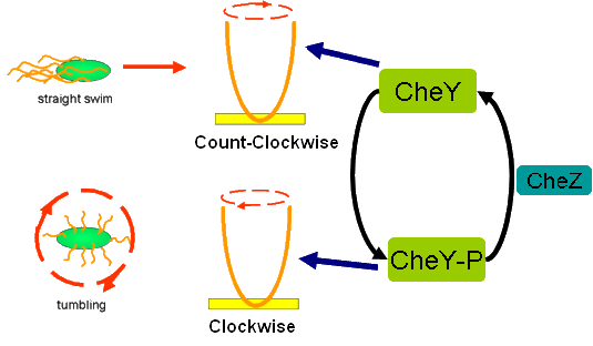
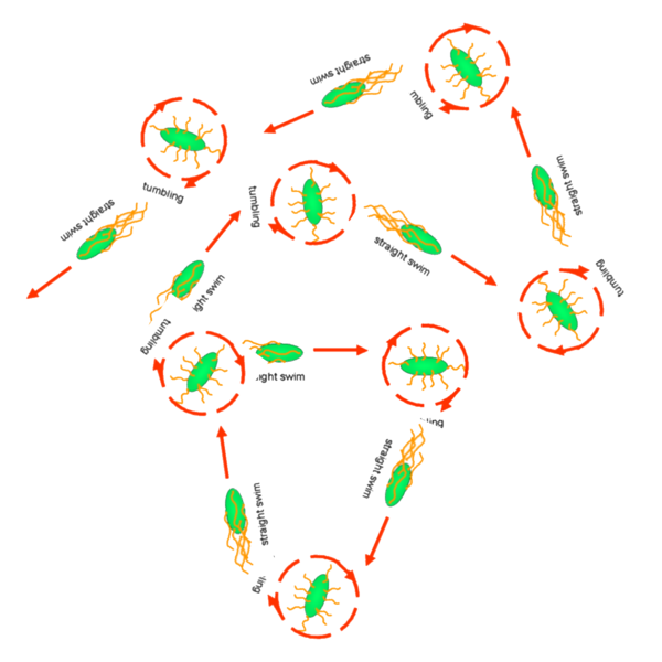
Cell Movement in Microscopic and Macroscopic AspectBasically, we considered the movement of a cell as a process of random walk, since an individual E.coli cell was always in the states between moving and tumbling (Fig.1).Similar to Brownian particles, the random walk of E.coli followed the Einstein-Smoluchowski theory [1].
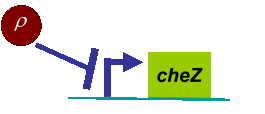
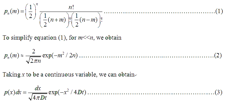
Fig . 1 Genetic circuit related to cell movementin(left) and cell random walk(right) Firstly, for the one dimension of random walk, let x (t) denote the position of an E.coli cell at time t, given that its position coincided with the point x=0 at time t=0. And we assumed an E.coli cell moves an average distance l—in either the positive or negative direction of the x-axis—each step (during a time (τ) between two tumbling states). The probability that the cell was found at the point x at time t was now equal to the probability that, in a series of n (=t/τ) successive moving steps, the cell made m more steps in the positive direction of the axis than in the negative direction. The desired probability was given by the binomial expression [1, 2]
where
v= l/τ was the average speed of the cell movement, and f=1/τ was the tumbling frequency of E.coli. In two dimensions, the square of the distance from the origin to the point (x, y) was r2=x2+y2; therefore For a macroscopic view, D was defined as the diffusion coefficient. Normally, as the swimming speed of E.coli is about 20um/s and the tumbling frequency is about 1 Hz, the diffusion coefficient is about 200um2/s [3].
Front propagation for cell growth
|
|
Fig. 2 The movie of the wild type pattern
in 2D(left) and 3D(right)
Density Dependent Motility
In experiments, we designed a circuit that the cell motility was repressed by cell density ρ. When the cell density ρ was high, the diffusion coefficient D became small. Therefore, the fisher’s equation as equation (4) was not valid in this case any more.
To order to be simplified, we firstly considered the one dimension problem again. We assumed the cell density at point x was ρ(x) at time t. In a very short time τ, there would be two groups of cell at x moving into its nearby points x-δ, x+δ, due to the random walk. And the amount of cell in each group were proportional to the product of D(ρ(x)) and ρ(x). Therefore,
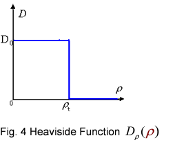
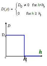
And the function Dρ(ρ) was a decrease function. For a simplest case, we considered a Heaviside Function
The numerical simulations gave us the results shown in Fig.5. The cell density showed a periodical-narrow-peak structure. These peaks were what we wanted, as they produced some regions of low cell density, though the whole pattern was not quite similar with that of experiments.
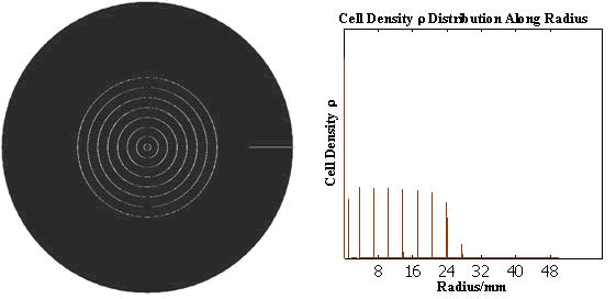
Fig. 5 Periodical-narrow-peak pattern in 2D(left);
the cell density distribution along the radius(right)
Full Model of Density Dependent Motility
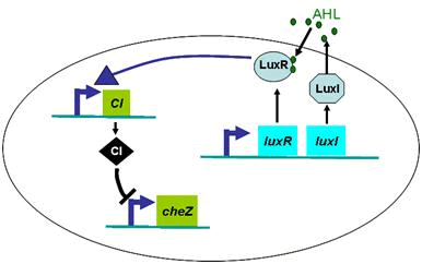
Actually, in our genetic circuit, we transformed a plasmid which can secrete AHL to environment (Fig.6). When the AHL density h of environment was high, the AHL came into the cell. Then AHL combining with LuxR repressed the expression level of cheZ which controled the motility of E.coli. So it was necessary to take account of the AHL effect.
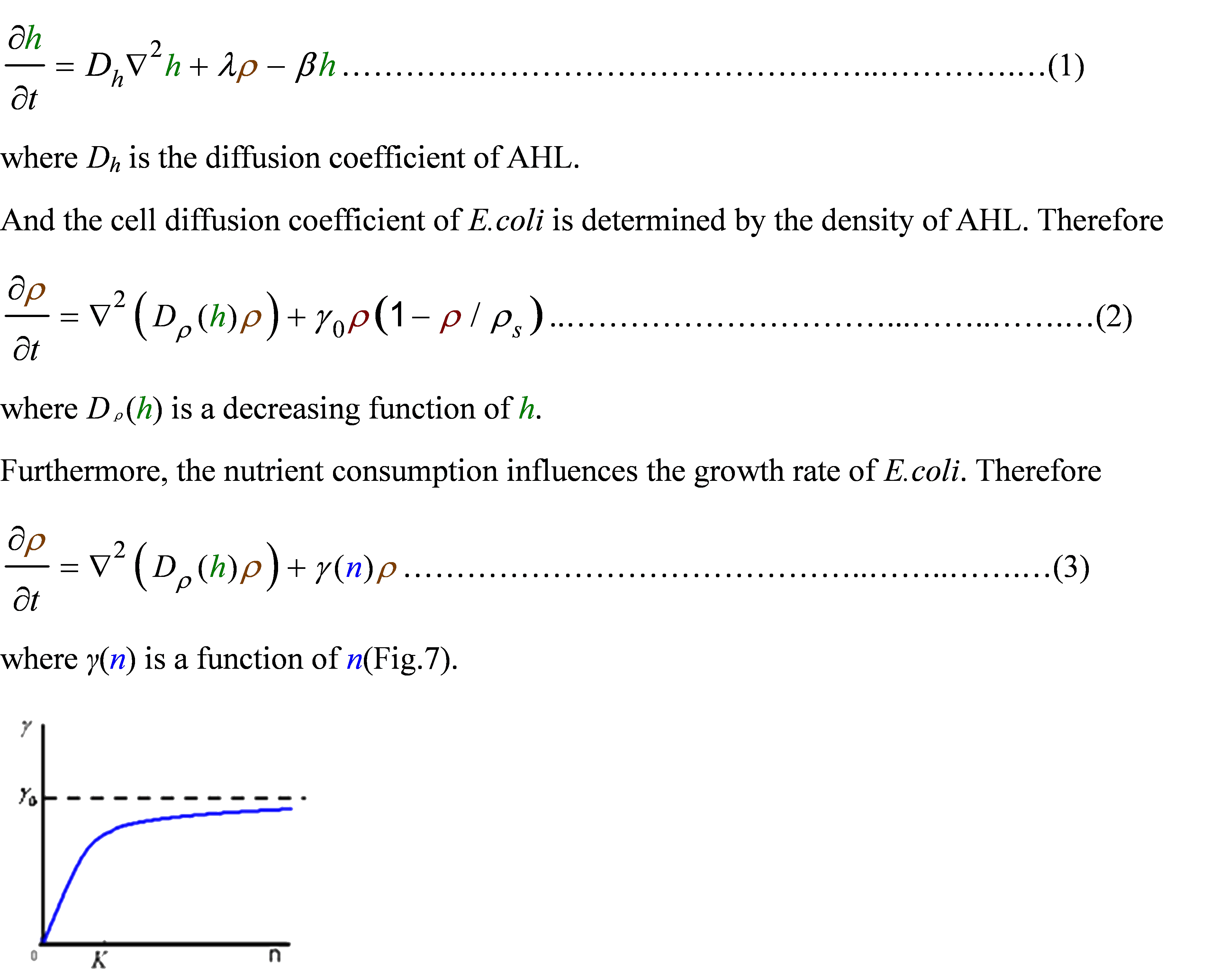
First, the AHL was synthesized by the E.coli cell at the rate λ. And the degradation rate β of AHL whose half life is normally about 15 to 30 minutes. Considering the diffusion of AHL, we obtained
For the nutrient, we made an assumption that the amount of nutrient consumed were proportional to the amount of cell increasing. Taking account of the nutrient diffusion, we had

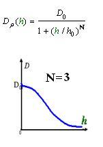
We used several possible forms of function Dρ(h)(see Results Section2). The results showed that if the cell diffusion coefficient decreases fast near the AHL density threshold, the pattern came out as a multiple-ring one(Results Section2 (a),(e)). On the contrary, there was only one-ring pattern.
Therefore, in order to to make this curve Dρ(h) decreasing sharply near the threshold, it followed a prediction that we can get a multiple-ring pattern by making an auto-activate genetic circuit which the combination of LuxR and AHL can activate the expression level of itself.
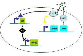
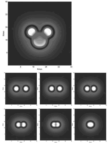
Furthermore, we did some two-spot patterns which initially have two points of E.coli cell, so as to compare with the experiments culture (Results Section3).
Results
We tried different parameters in the model, to see how they influenced the pattern.
Generally, we can vary the parameters of cell growth and cell motility which, in experiments, are easy to change, although there are lots of parameters in our model. So we list the results of varying several parameters in the cell growth part and cell motility part.
1. Cell Growth
In the cell growth term, we considered the growth rate was related to nutrient concentration. When the nutrient was consumed by the cell, the grow rate of the cell would decrease (Fig. 7). There was a maximum growth rate γ0, when the nutrient was rich. The parameter κ described the sharp of this curve(Fig. 7). The larger κ gave us more smooth increasing curve. And we made an assumption that one unit of nutrient would change to cell number with a ratio α. Also in the initial condition, the nutrient concentration ni can influence the patterns. Therefore, the effects of all the four parameters were studied in our model.
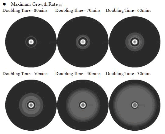
Above reuslts indicated that, the faster cell growth (larger γ0 and smaller doubling time) formed a smaller and a little more unclear ring pattern. And the inner ring diameter would become a litter more large when the growth rate increased.
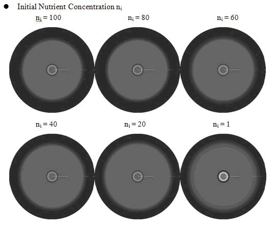
From above figures, it was found that the initial nutrient concentration ni had little influence to the pattern, especially when it was large. The only effect we observed was that smaller initial nutrient concentration ni made the ring slightly wider and more clear.
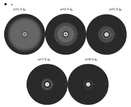
Here, the value of κ was related to the initial nutrient concentration ni. When initial nutrient concentration ni was fixed, a smaller κ parameter gave us the similar results with that of faster cell growth.
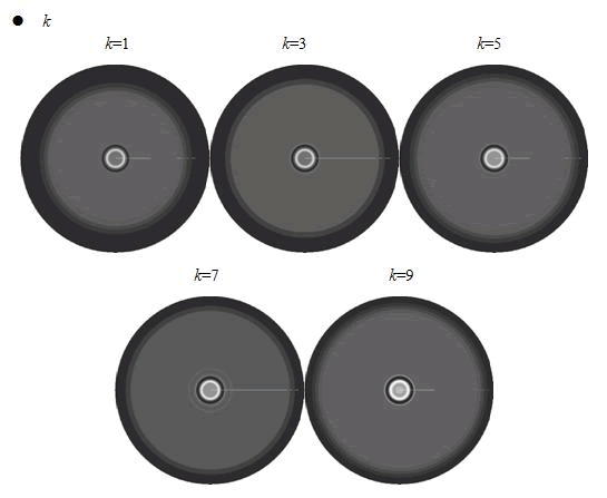
When we increased the value of k, the patterns did not change a lot, but only became a little more clearly.
In conclusion, the simulation results showed that the parameters of maximum growth rate γ0 and κ had a more important role on the ring-like pattern. And the other two parameters k and ni did not influence the pattern much.
2. Cell Motility Dρ(h)
As Dρ(h) was a decreasing function of h, the possible formed of it can be
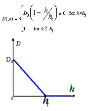 |
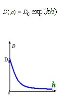 |
 |
 |
Click graph to see movie!~(Line 1 left to right a, b, c; Line 2 left to right d ,e )
With the initial conditions of two or more spots, we obtained the below funny patterns which are amazing similar with that of experiments(results).
- [1] P.K.Pathria, Statistical Mechanics (Pergamon Press, Headington Hill Hall, Oxford; 1972)
- [2] Howard C.Berg, Random Walks in Biology (Princeton University Press, Princeton, Hew Jersey; 1993)
- [3] Nikhil Mittal, et al, Proc Natl Acad Sci 100, 13259 (2003)
- [4] R. A. Fisher, Ann. Eugenics 7, 353 (1937)
- [5] A.H.Bokhari, et al., Nonlinear Analysis (In Press)
---------------------------------------------------------------------------------------------
 |
 |
 |
 |
 |
 "
"
 ,
, 