Team:Paris/Modeling/BOB
From 2008.igem.org
(→Normalization) |
|||
| Line 81: | Line 81: | ||
[[Image:Beta_p_Resize.jpg|center]] | [[Image:Beta_p_Resize.jpg|center]] | ||
<br> | <br> | ||
| - | In fact, if we take CFP for example: | + | * In fact, if we take CFP for example: |
[[Image:CFP.jpg|center]] | [[Image:CFP.jpg|center]] | ||
If we set [fliA] = 1 and [flhDC] = 1, and we solve, we obtain : | If we set [fliA] = 1 and [flhDC] = 1, and we solve, we obtain : | ||
| Line 87: | Line 87: | ||
Setting the equilibrium value to 1 corresponds to setting | Setting the equilibrium value to 1 corresponds to setting | ||
[[Image:Beta_Gamma_resize.jpg|center]] | [[Image:Beta_Gamma_resize.jpg|center]] | ||
| - | The analysis of fliA is different, but not the result: | + | * The analysis of fliA is different, but not the result: |
[[Image:FliA_Analysis.jpg|center]] | [[Image:FliA_Analysis.jpg|center]] | ||
With an input of flhDC equal to 1, the solution of the differential equation is: | With an input of flhDC equal to 1, the solution of the differential equation is: | ||
| Line 93: | Line 93: | ||
And the condition on the equilibrium imposes | And the condition on the equilibrium imposes | ||
[[Image:Beta_Gamma_Resize_FliA.jpg|center]] | [[Image:Beta_Gamma_Resize_FliA.jpg|center]] | ||
| - | To conclude, we see that we always get the same condition: | + | * To conclude, we see that we always get the same condition: |
[[Image:Final_Resize.jpg|center]] | [[Image:Final_Resize.jpg|center]] | ||
| - | Finally, since we had imposed γ=1 we resulted with β+β | + | * Finally, since we had imposed γ=1 we resulted with β+β'=1. |
==== Which gene goes were? ==== | ==== Which gene goes were? ==== | ||
Revision as of 17:09, 27 August 2008
Introduction
Steps modeledHere is a quick summary of the step we decided to interpret mathematically:
Establishing the modelPopulation evolution
FIFO Temporal Order ModuleSteps involved
Mathematical model
DiscussionNormalization
If we set [fliA] = 1 and [flhDC] = 1, and we solve, we obtain : Setting the equilibrium value to 1 corresponds to setting
With an input of flhDC equal to 1, the solution of the differential equation is: And the condition on the equilibrium imposes
Which gene goes were?Synchronization ModuleSteps involved
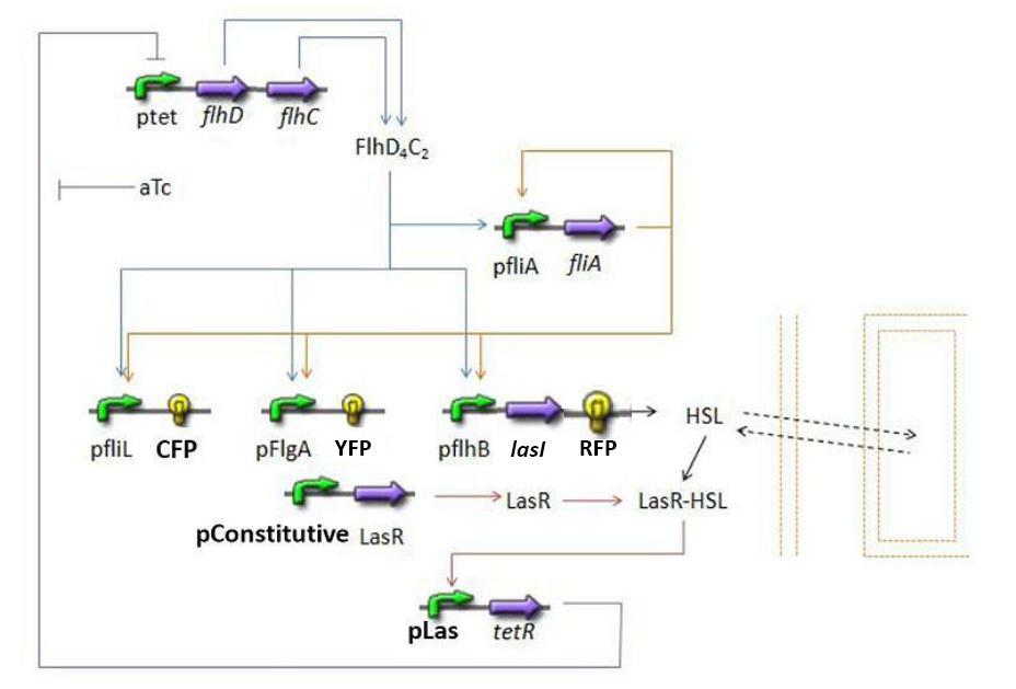
Mathematical ModelDynamics of HSLDynamics of HSLextTetR=f(HSL)FlhDC=f(TetR)fliA = f(FlhDC,FliA) (1) RFP and lasI behind pFliL = f(FlhDC,FliA) (2) Influence of lasI over HSL (3) Relation between HSL and HSLext (4) Influence of HSL over tetR (5) flhDC = f(tetR) (6) 4.3.2 Mathematical model First of all, we naturally keep the same model for steps (1) and (2). 4.3.2.1 Dynamics of HSL First and foremost, HSL is the key element in the synchronization process. We used a diffusive specie in order to balance the concentrations between cells. The outside medium concentration becomes an intermediate variable. We ended with
Where is the diffusion rate expressed in time-1 and
Then, we had two choices to model this step. At first we were inspired by [2] where the production of HSLint is described as being linear, and we were given the value of the constant. However, the results presented in this study were introduced as only being theoretical. The degradation rate comes in quite naturally.
We chose to model the creation of HSL by a Michaelis Menten expression. In fact, we found out that lasI seemed to be a monomeric enzyme, thus setting the Hill parameter to 1.
Here, is expressed in the concentration unit, and in the concentration unit by time unit. It is important to note that we took into account the fact that lasR/(lasR linked to HSL) was a function of HSL. However, we assumed that the fraction of HSL bound to lasR would not influence HSL concentration; this is the reason why, no “degradation due to binding term” appears in the HSL model. 4.3.2.2 Dynamics of HSLext The evolution of HSLext may be described with three terms. First of all, there is a dilution rate, Drenewal, due to the renewal of the chemostat. There is the usual degradation rate, .
Which gives
4.3.2.3 TetR = f(HSL) Here we had the choice to model the complexation phase of HSL and lasR, and then the binding phase of this complex on the pLas promoter. We assumed that those stages were short, and then decided to model them by a single step.
We checked in the registry that the pLas sequence was the same as in [promoter specificity]. It is explained that there are two operators, denoted OP1 and OP2. The Hill parameters were detailed in this article, hence our modeling choice : Oscillations ModuleFlhDC = f(TetR) For this last step, since we have not found any article indicating that we could simplify the model by using a linear function. Then, we chose a complete Hill function to describe the dynamics of flhDC: Parameters summaryResultsBibliographyMuch of our inspiration comes from four articles to which we shall refer in the next subsections :
|
 "
"

