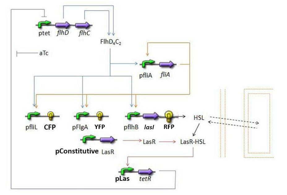
Introduction

The key problem with a dynamic system consists in the fact that adding a new equation gives a more detailed idea of the overall process, but one looses meaning by doing so since new undefined parameters appear. Hence, it becomes hard to link those parameters with a biological meaning and reality.

In that respect we chose to build at first a simplified model, which would enable us to help us understand the processes implied in the system. In that respect, we chose not to introduce the mRNA state between transcription and translation in our model. We presented things as if a protein would act directly upon the following. Furthermore, we assumed that describing routinely every step, would only force us into finding more parameters.

This preliminary approach is mainly based on a bibliographical work. In fact, it is important to understand that with this approach, we did not intend to design the most accurate model possible. We found essential to choose only parameters that we could determine or control in the wet lab. The main goal was to get quickly a first idea of the way our system could behave.

The goal here is to present the differential equations we used in the model. At each step we shall describe why we chose these precise equations, the drawbacks and possible improvements, the parameters involved and eventually a biologically coherent value.

Steps of the Model

Here is a quick summary of the step we decided to interpret mathematically:

FIFO Temporal Order module

• FliA behind pFliA= f(FlhDC,FliA)
• CFP behind pFliL = f(FlhDC,FliA)
• YFP behind pFliL = f(FlhDC,FliA)
• RFP and LasI behind pFliL = f(FlhDC,FliA)

Synchronisation module

• HSL = f(LasI) or f(LuxI) depending on which system is being used
• HSL ⇋ HSLext
• TetR = f(HSL)

Oscillations module

• FlhDC = f(TetR)

Establishing the model

Population evolution

• First of all, it seems important at this stage to present the way we interpret the evolution of the population in the chemostat. We want to impose to our model the fact that the rate of production has to be proportional to the existing population and to the amount of available resources. Hence a logistic model of the population, where c denotes the concentration of cells in the medium:

• Then, we need to add the death term, and a dilution term cause by the renewal of the chemostat. Finally we get :

where c_max is the carrying capacity for cell growth, and D the dilution rate, d the death rate constant

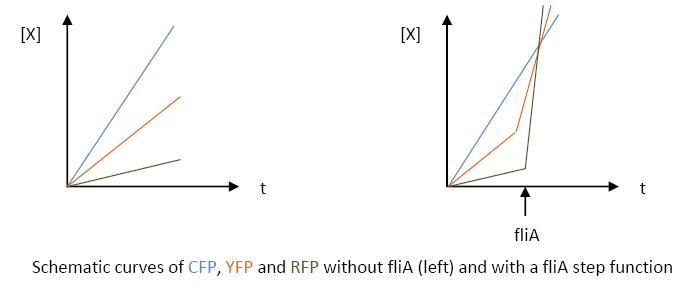
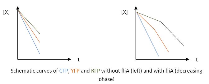
FIFO Temporal Order Module

Steps involved

• FliA behind pFliA= f(FlhDC,FliA)
• CFP behind pFliL = f(FlhDC,FliA)
• YFP behind pFliL = f(FlhDC,FliA)
• RFP and LasI behind pFliL = f(FlhDC,FliA)

Mathematical model

• Classically we use the following equation to model gene interactions :

where [Y] denotes the concentration of Y protein and γ its degradation rate (which unit is time^-1).

• Yet, the flagella gene network has been thoroughly studied in [1]. We used two major results presented in this study. Firstly, Shiraz Kalir and Uri Alon came up with the fact that the promoters of class 2 genes, among which fliL, flgA and flhB, behaved like SUM-gate functions with flhDC and fliA inputs. Secondly, their experiments proved that these influences could be considered as linear. Thus the following model:

β and β’ represent the relative influence of flhDC and fliA respectively, the units of β and β’ being time^-1.

• Furthermore, they came up with numerical values of β and β’ for each gene, which fitted quite well to their experiments. We then decided that we could use those values as well in our model.

• Finally, here are our final equations:

Discussion

Normalization

• First of all, we wanted to have a proper time scale. We the set the degradation rates, γ ,to 1. It is important to note that this degradation rate is represent the influence of the degradation and dilution. We assume that the degradation is insignificant compared to the dilution. Then we have:

• Since we can know easily the value of the real half-time, we may know the real timescale out of our computations. We kept the designation “degradation rate” for convenience, so as not to mix up with the dilution that occurs with the HSL in the synchronization step.
• We kept the β and β’ values found by S. Kalir and U. Alon, since they showed the relative influence of flhDC and fliA. To have the same order of magnitude between each specie, we normalized those parameters between 0 and 1 as following. We reasoned independently for each equation, wishing to set the equilibrium values of the concentration to 1 given input values of 1. This gave:

• In fact, if we take CFP for example:

If we set [fliA] = 1 and [flhDC] = 1, and we solve, we obtain :

Setting the equilibrium value to 1 corresponds to setting

• The analysis of fliA is different, but not the result:

With an input of flhDC equal to 1, the solution of the differential equation is:

And the condition on the equilibrium imposes

• To conclude, we see that we always get the same condition:

• Finally, since we had imposed γ=1 we resulted with β+β'=1.

Which gene goes were?

• The key element to understand is that fliA stands as an accelerator. The first influence is caused by flhDC, and fliA gives the last burst. fliA also has a great influence in the fading phase, since it introduces a delay (result found by experiments in [1]). This is what determined our choice in the order of fliL, flgA and flhB. We wanted to put in first the gene that was the least influenced by fliA, and in the end the gene the most influenced by fliA.

• In fact, this enabled us to force the curves into crossing themselves. In addition, the delay imposed by fliA in the decreasing phase, would permit us to widen the delays between the first and the last gene expression, thus getting better conditions to observe the FIFO in the wet lab.

Synchronization Module

Steps involved

• HSL = f(LasI) or f(LuxI) depending on which system is being used
• HSL ⇋ HSLext
• TetR = f(HSL)

Mathematical Model

Dynamics of HSL

First and foremost, HSL is the key element in the synchronization process: we used a diffusive specie in order to balance a value between cells. Thus, the HSL concentration denoted [HSL] become this "shared" value, the outside medium concentration denoted [HSL_ext] being an intermediate value.

We use the classical osmosis term η x ( [HSL] - [HSL_ext] ) where η = membrane permeability x ( area _1cell / volume _1cell ) is the diffusion rate expressed in time^-1.

The degradation rate is linear: - γ x [HSL].

To model the production, we were at first inspired by [2] where it is described as being linear: β x [LasI] where β is a given constant value. However, the results presented in this study were introduced as only being theoretical so we chose to model the creation of HSL by a Michaelis Menten expression (it can be seen as a Hill expression where the Hill parameter is set to 1 because of LasI seeming to be a monomeric enzyme).

It is important to note that we took into account the fact that lasR/(lasR linked to HSL) was a function of HSL. However, we assumed that the fraction of HSL bound to lasR would not influence HSL concentration; this is the reason why, no “degradation due to binding" term appears in the HSL model.

Dynamics of HSL_ext

The evolution of HSLext may be described with three terms. First of all, there is a dilution rate, D_renewal, due to the renewal of the chemostat. There is the usual degradation rate,γ_[HSL]ext ).

Which gives

where

TetR=f(HSL)

• Here we had the choice to model the complexation phase of HSL and lasR, and then the binding phase of this complex on the pLas promoter. We assumed that those stages were short, and then decided to model them by a single step.

• We checked in the registry that the pLas sequence was the same as in [promoter specificity]. It is explained that there are two operators, denoted OP1 and OP2. The Hill parameters were detailed in this article, hence our modeling choice :

Oscillations Module

FlhDC = f(TetR) For this last step, since we have not found any article indicating that we could simplify the model by using a linear function. Then, we chose a complete Hill function to describe the dynamics of flhDC:

Parameters summary

(Under Construction)

Bibliography

Much of our inspiration comes from four articles to which we shall refer in the next subsections :

• [1] Shiraz Kalir, Uri Alon. Using quantitative blueprint to reprogram the dynamics of the flagella network. Cell, June 11, 2004, Vol.117, 713-720.
• [2]Jordi Garcia-Ojalvo, Michael B. Elowitz, Steven H. Strogratz. Modeling a synthetic multicellular clock : repressilators coupled by quorum sensing. PNAS, July 27, 2004, Vol. 101, no. 30.
• [3]Frederick K. Balagaddé, Hao Song, Jun Ozaki, Cynthia H. Collins, Matthew Barnet, Frances H. Arnold, Stephen R. Quake, Lingchong You. A Synthetic Escherichia Coli predator prey ecosystem. Molecular Systems Biology. 2008.

A VOIR

• [3]Nitzan Rosenfeld, Uri Alon. Response delays and the structure of transcription networks. JMB, 2003, 329, 645-654.
• [4]Nitzan Rosenfeld, Michael B. Elowitz, Uri Alon. Negative autoregulation speeds the response times of transcription networks. JMB, 2003, 323, 785-793.
• [5]S.Kalir, J. McClure, K. Pabbaraju, C. Southward, M. Ronen, S. Leibler, M. G. Surette, U. Alon. Ordering genes in a flagella pathway by analysis of expression kinetics from living bacteria. Science, June 2001, Vol 292.