An Oscillatory Biological Model
Introduction
- The goal here is to present the differential equations we used in the system modelization. At each step, we shall describe why we chose this precise model, its drawbacks and possible improvments, the parameters involved and enventually a biologically coherent value.
- The key problem with a dynamic system consists in the fact that adding a new equation gives a more detailed idea of the overall process, but one looses precision by doing so since new parameters appear.
- In that respect (in all cases but one) we chose not to model the mRNA steps, that is translation and transcription. We then assumed that we could act as if a protein would directly act upon the follower, without loosing too much precision. We attached a lot of importance to describing only interaction for which we could find values in the article. Furthermore we assumed that describing routinely the mRNA step would force us into finding more parameters and thus loosing precision.
- This first approach refers to a set of two cells. We shall examine later on what happens if we put more cells together.
- It seems important to understand that with this approach, we did not intend to design the most accurate model possible. We found essential to chose only parameters that we could determine and command in the wet lab. The main goal was to get quickly a first idea of the way our system could behave.
Bibliography
Much of our inspiration comes from four articles to which we shall refer in the next subsections :
- [1] Shiraz Kalir, Uri Alon. Using quantitative blueprint to reprogram the dynamics of the flagella network. Cell, June 11, 2004, Vol.117, 713-720.
- [2]Jordi Garcia-Ojalvo, Michael B. Elowitz, Steven H. Strogratz. Modeling a synthetic multicellular clock : repressilators coupled by quorum sensing. PNAS, July 27, 2004, Vol. 101, no. 30.
- [3]Nitzan Rosenfeld, Uri Alon. Response delays and the structure of transcription networks. JMB, 2003, 329, 645-654.
- [4]Nitzan Rosenfeld, Michael B. Elowitz, Uri Alon. Negative autoregulation speeds the response times of transcription networks. JMB, 2003, 323, 785-793.
- [5]S.Kalir, J. McClure, K. Pabbaraju, C. Southward, M. Ronen, S. Leibler, M. G. Surette, U. Alon. Ordering genes in a flagella pathway by analysis of expression kinetics from living bacteria. Science, June 2001, Vol 292.
Summary of the steps modelized
- Here is a quick summary of the interactions we decided to interpret mathematically...
- Influence of flhDC over fliA
- Influence of flhDC and fliA over fliL - Fluorescent Protein 1 (FP1)
- Influence of flhDC and fliA over flgA - Fluorescent Protein 2 (FP2)
- Influence of flhDC and fliA over flhB - Fluorescent Protein 3 (FP3)
- Influence of flhDC and fliA over flhB - lasI
- Influence of lasI over HSLint
- Relation between HSLint and HSLext
- Influence of HSLint over tetR mRNA
- Influence of tetR mRNA over tet R
- Influence of tetR over flhDC
Establishing the model
- Steps
- Influence of flhDC over fliA
- Influence of flhDC and fliA over fliL - Fluorescent Protein 1 (FP1)
- Influence of flhDC and fliA over flgA - Fluorescent Protein 2 (FP2)
- Influence of flhDC and fliA over flhB - Fluorescent Protein 3 (FP3)
- Influence of flhDC and fliA over flhB - lasI
The transcription hierarchy of the flagella class2 gene network has been thoroughly studied in [1]. It resulted that the promoter activity of fLiL, flgA, flhB, may be mathematically described in that way :
where [X] denotes the effective protein-level activity.
In fact, they proved that the effects of fliA and flhDC were additive. The goal of this mathematical approach is then to characterize this highly interesting result.
For each gene, Shiraz Kalir and Uri Alon came up with numerical values of β and β', available in [1].
Furthermore, the protein-level activity can be presented (for a more detailed presentation, see [4]) as
Thus :
- Discution and Asumptions
- As presented in the first equation below, there is a retroaction from fliA over fliA. In a first approach, we decided not to take into account this interaction, that is setting β'FliA to zero. In a second approach, we will consider this retroaction, and find a way to describe it mathematically.
- Another step consists in choosing the proper units, so as to have a homogenous set of parameters.
- Finally, it is important to understand at this stage the choice we made when we decided to present this model. Our goal was to have a rough but somehow realistic (i.e. grounded on studies available on the literature) model with which we could start to work, for example to have an idea of time scales. This is the reason why we ended with this linear appproach grounded on a bibliographic approach.
- Steps
- Influence of lasI over HSLint
- Relation between HSLint and HSLext
- Mathematical model
Furthermore, when considering more than one cell, we shall use this model :
- Here, we assumed that we had a homogenous growth medium.
- This model for HSL<int> evolution is quite straight forward. There is a production term, proportional to the gene that is the source for its creation, and a degradation term proportional to the concentration of HSL<int> itself. Then, HSL goes in and out of the cell. The third term in the equation describes then the diffusion which is commonly described thanks to a dynamical study :
- Then we assumed that δext could be well modelized by the mean of the δint of each cell.
- Discution and Asumptions
- In a first approach, we have assumed that HSL could be modelized in the same fashion as AHL. The process was well detailed in [2] and we adapted their model to our present situation. Furthermore, a biologically coherent set of parameters is also given in this article. We decided then to use them as well for our simulation.
- Steps
- Influence of HSLint over tetR mRNA
- Influence of tetR mRNA over tet R
- Discution and Asumptions
- Here is the only case where we have not yet found out how we could manage to skip the mRNA step. However, this is acceptable since every parameter should be available. Then, (12) represents the binding and transcription steps ; (13) represents the translation step.
- The effect of HSL as well as the link between the mRNA activity and protein activity is well studied in [2]. We were the able to adapt the introduced situation to our system.
- The ρ parameter corresponds to maximal contribution to tetR transcription in presence of saturating amounts of HSL. Yet, to begin with, we have used the parameter given in the text. We shall then find a more accurate parameter corresponding to our system. The HSL activation is hereby chosen to follow Michalelis Menten kinetics since we assumed that there would be no cooperativity.
- Finally, we assumed that lasR would exist permanently in the medium in sufficient amounts, so that we needn't take it into account mathematically speaking.
- Steps
- Influence of tetR over flhDC
F is a threshold function: F(tetR)=(∆/2)*(1+(τ-tetR)/sqrt((tetR-τ)^2)),
τ being the threshold and ∆ being the activity before repression.
- Discution and Asumptions
- To determine this part of the model, we used [4] where the influence of tetR is described.
- Finally, to close the loop, we saw the necessity to use a little refinment. the influence of tetR over pTet (pTet being the promoter of flhDC) is a repression. To express the fact that a certain concentration is needed for the expression of flhDC, we used a step function. This choice was influenced by [3]. To fully define this function, two parameters are needed, so as to describe the threshold when the step has to occur, and the initial value of this step. We are facing two solutions. The more accurate procedure would consist in getting those values from the wet-lab. However, we may also look it up in the literature. Anyhow, as presented in the conclusive part, there is a really wide range of parameters that enable the system to oscillate.
- The key problem was that those two parameters were to be determined by the overall evolution of tetR, and the program cannot wait for tetR to be entirely determined to evaluate flhDC, since we have a loop. We then decided that these parameters could be obtanied by lab experiments.
Parameters summary
- Awaiting for experimental values, since it seemed coherent by reading articles, we have chosen to set every degradation rate to 1.
| Parameter Table
|
| Parameter
| Parameter in code (cell i)
| Meaning
| Value
| Unit
| Source
| Accuracy
| Comments
|
| γFliA
| g[1 + 8 x (i-1)]
| Degradation rate
| 1
|
| [1]
|
|
|
| βFliA
| B(1,i)
| FlhDC activation coefficient
| 50
|
| [1]
|
|
|
| β'FliA
| b(1,i)
| FliA activation coefficient
| 0
|
| [1]
|
|
|
| γFP1
| g[2 + 8 x (i-1)]
| Degradation rate
| 1
|
| [1]
|
|
|
| βFP1
| B(2,i)
| FlhDC activation coefficient
| 1200
|
| [1]
|
|
|
| β'FP1
| b(2,i)
| FliA activation coefficient
| 250
|
| [1]
|
|
|
| γFP2
| g[3 + 8 x (i-1)]
| Degradation rate
| 1
|
| [1]
|
|
|
| βFP2
| B(3,i)
| FlhDC activation coefficient
| 150
|
| [1]
|
|
|
| β'FP2
| b(3,i)
| FliA activation coefficient
| 300
|
| [1]
|
|
|
| γFP3
| g[4 + 8 x (i-1)]
| Degradation rate
| 1
|
| [1]
|
|
|
| βFP3
| B(4,i)
| FlhDC activation coefficient
| 100
|
| [1]
|
|
|
| β'FP3
| b(4,i)
| FliA activation coefficient
| 350
|
| [1]
|
|
|
| γlasI
| g[4 + 8 x (i-1)]
| Degradation rate
| 1
|
| [1]
|
|
|
| βlasI
| B(4,i)
| FlhDC activation coefficient
| 100
|
| [1]
|
|
|
| β'lasI
| b(4,i)
| FliA activation coefficient
| 350
|
| [1]
|
|
|
γHSLint
| g[5 + 8 x (i-1)]
| Degradation rate
| 1
|
| [1]
|
|
|
βHSLint
| B(5,i)
| Production rate
| 0,01
|
| [2]
|
|
|
| δint
| D(1,i)
| Diffusion rate in the cell
| 2
|
| [2]
|
|
|
γHSLext
| g[6 + 8 x (i-1)]
| Degradation rate
| 1
|
| [1]
|
|
|
| δext
| D(2,i)
| Diffusion rate out off the cell
| 2
|
| [2]
|
|
|
| γtetR mRNA
| g[6 + 8 x (i-1)]
| Degradation rate
| 1
|
| [1]
|
|
|
| ρ
| R(i)
| Maximal contribution to tetR in the presence of saturating amounts of HSL
| 20
|
| [2]
|
|
|
| θ
| 0(i)
| Ratio between mRNA and protein lifetimes
| 1
|
| [2]
|
|
|
| γflhDC
| g[8 + 8 x (i-1)]
| Degradation rate
| 1
|
| [1]
|
|
|
| τ
| T(i)
| Threshold for tetR repression
| (20000)
|
| lab
|
|
|
| ∆
| Pa(i)
| Promoter activity without the repressor
| (100)
|
| lab
|
|
|
Screenshots and graph description
- We presented this model as being rough but functional. These graphs show a set of first results we managed to get. We directly put our results concerning two cells. The goal is to present the overall behavior of the system, according to the linear model.
- As far as the initial condition are concerned, we decided to run the simulation with null conditions of every specie, but for flhDC since flhDC is due to appear as the starter of our cycles. We tried to change the initial input in flhDC, but the system proved capable of robustness towards the diferent values we chose. Except for the amplitude of the oscillation, the overall behavior of the system remained constant.
- The FIFO behavior is not yet obvious, if we keep the parameters we found in the articles. Though, by zooming precisely on the curves, and following them we may see that a FIFO behavior is occuring. We shall quantify later what FIFO characteristics we decide impose to the system. That is what we have described so far as a glimpse of FIFO.
- When various cells are introduced, we wanted them not to behave exactly as the first cell. When then introduced a noise function, that sets randomly the parameters of the others cells between 90% and 110% of those of the first reference cell.
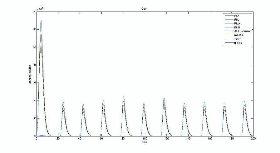 Cell1 in a 2 cells model : oscillations and a glimpse of FIFO Cell1 in a 2 cells model : oscillations and a glimpse of FIFO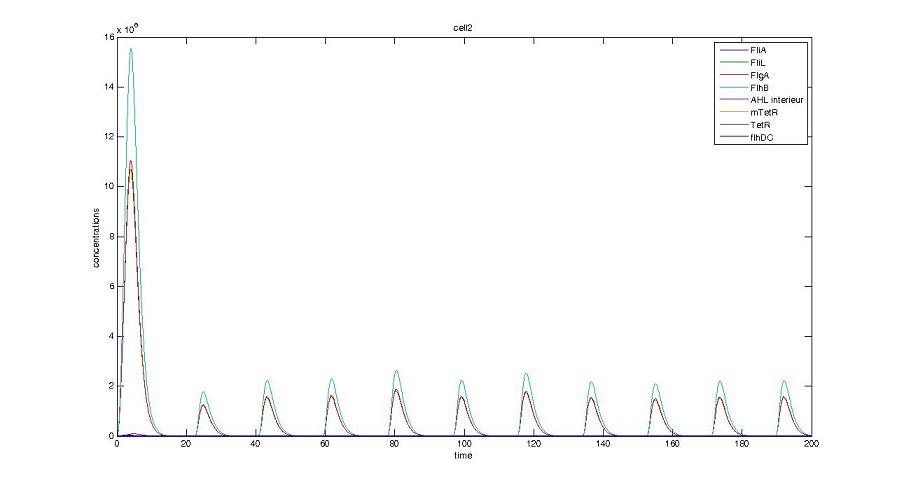 Cell2 (noise added to set the parameters) in a 2 cells model : oscillations and a glimpse of FIFO Cell2 (noise added to set the parameters) in a 2 cells model : oscillations and a glimpse of FIFO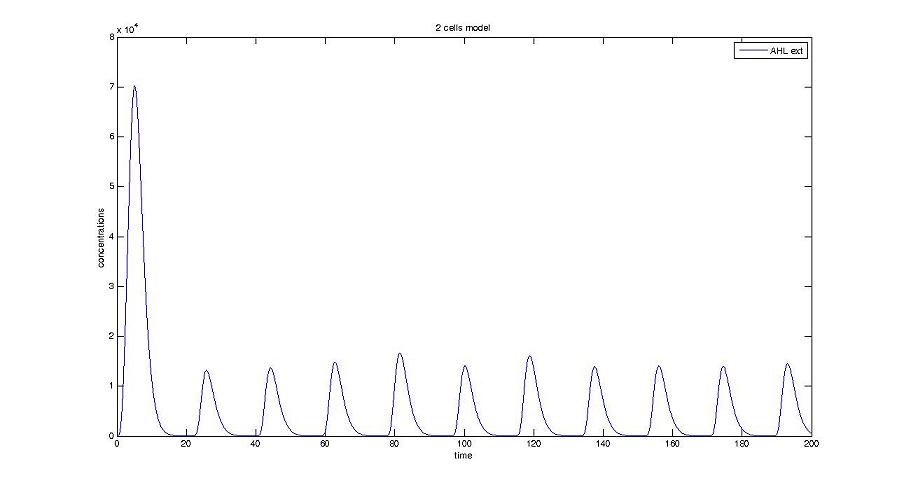 HSL ext in a 2 cells model : oscillations HSL ext in a 2 cells model : oscillations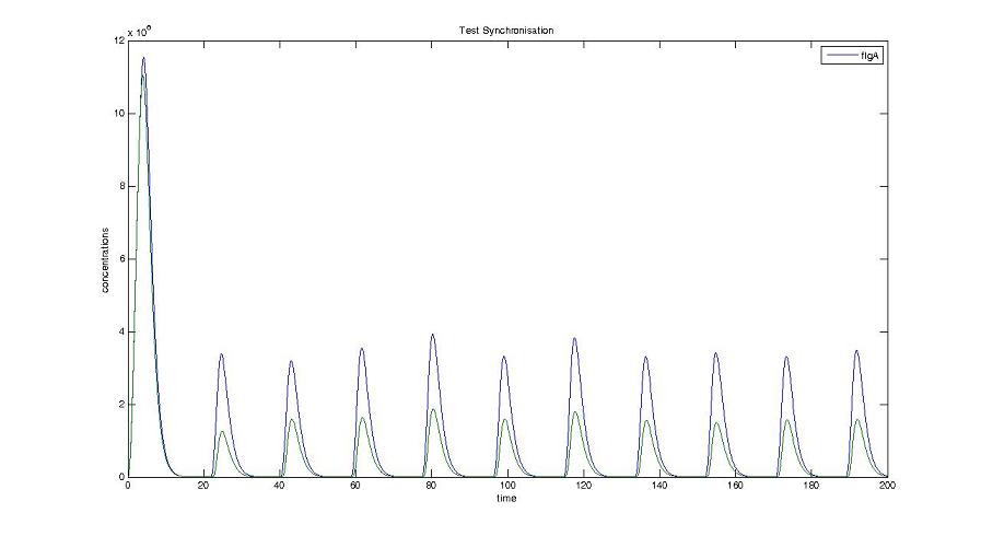 Synchronisation : flgA in both cells Synchronisation : flgA in both cells Synchronisation : fliL in both cells Synchronisation : fliL in both cells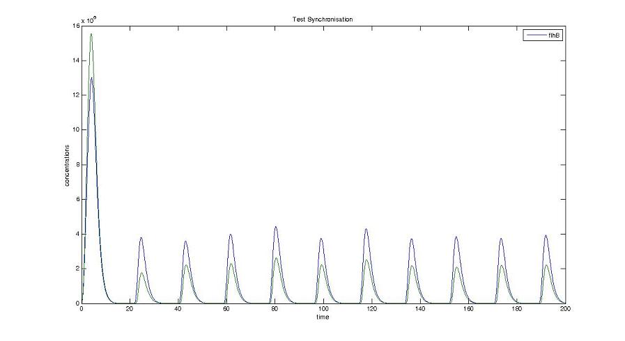 Synchronisation : flhB in both cells Synchronisation : flhB in both cells Corresponding codes
- To change the parameters, you have to use this file, and refer to the previous array : Model
- To launch the numerical simulation and plot the curves : Plot the curves
- To compute the numerical simulations (does not provide any visual output, but necessary for the previous script) : Numerical simulations
- To add noise to deterministic parameters : Noise function
- To define all the parameters in a row : Parameters
<a href=http://prix-ciajis-generique.com/>vente cialis</a> cialis generique
Concerning the parameters taken from [2], it has to be noticed that output units are arbitrary. Nonetheless, as the degradation rate is also 1, as in [1], one can infer that the transformations (to obtain the 'real' time and Fluorescence units) are the same in [2] than in [1].
Thanks to those assumptions, we are finally ended up with a quantitative description of the biological system, instead of just a qualitative one.
|
 "
"


