Team:Montreal/Modeling
From 2008.igem.org
(new, improved rate of external reaction) |
(Removing one of the three AI plot.) |
||
| (32 intermediate revisions not shown) | |||
| Line 9: | Line 9: | ||
!style="text-align:center; background-color:#cd0000; border-width:0px; padding:3px;"|[[Team:Montreal/Sponsors|<font color="#ffffff">Sponsors</font>]] | !style="text-align:center; background-color:#cd0000; border-width:0px; padding:3px;"|[[Team:Montreal/Sponsors|<font color="#ffffff">Sponsors</font>]] | ||
|} | |} | ||
| - | |||
| - | |||
===Background=== | ===Background=== | ||
| - | [[Image:Theoteam1.jpg|thumb|Theorists: Vincent Quenneville-Bélair and Alexandra Ortan|right|300 px ]] | + | [[Image:Theoteam1.jpg|thumb|Theorists: Vincent Quenneville-Bélair and Alexandra Ortan|right|300 px]] |
| - | Using coupled differential equations, we are modeling the Repressilator, which is a | + | Using coupled differential equations, we are modeling the Repressilator network, which is a composed of three genes, whose product proteins are repressing each other's growth. This cycle is taking place in each of a colony of cells, who communicate amongst themselves by exchanging an autoinducer molecule (AI, or PX here). The model attempts to take into account a sparse, heterogeneous distribution of many cells (grouped in clusters) with depletion of the autoinducer molecule and leakage while assuming continuous levels of the different proteins, as well as a continuous spatial distribution of these proteins. |
| - | For this purpose, the model is currently being coded up in Mathematica. The simulations, based on that continuous model, are generated using xCellerator and NDelayDSolve for different cell configurations (fig. 1); the results obtained are graphs of the concentration of molecules in the system versus time (fig. 2). That is, our interest lies in understanding the behaviour of the clusters with respect to each other (for instance, the phase difference or the synchronization time as in fig. 4-5). As of now, a low number (~4) of cells in two clusters is being used for testing, but a higher one (>100) in more clusters will be reached later. | + | For this purpose, the model is currently being coded up in Mathematica. The simulations, based on that continuous model, are generated using xCellerator [1] and NDelayDSolve for different cell configurations (fig. 1); the results obtained are graphs of the concentration of molecules in the system versus time (fig. 2). That is, our interest lies in understanding the behaviour of the clusters with respect to each other (for instance, the phase difference or the synchronization time as in fig. 4-5). As of now, a low number (~4) of cells in two clusters is being used for testing, but a higher one (>100) in more clusters will be reached later. |
===The Model=== | ===The Model=== | ||
| - | For the interested reader, the system of differential equations for the Repressillator network is composed of internal and external reaction. The internal reactions model | + | For the interested reader, the system of differential equations for the Repressillator network is composed of internal and external reaction. X, Y and Z are mRNA's and PX, PY and PZ their respectively associated product proteins. AI is assumed to be the same as PX. The internal reactions model what happens inside a cell and the equations are |
| - | |||
PY<sub>i</sub>'(t) = -βPY<sub>i</sub>(t) + βY<sub>i</sub>(t) | PY<sub>i</sub>'(t) = -βPY<sub>i</sub>(t) + βY<sub>i</sub>(t) | ||
PZ<sub>i</sub>'(t) = -βPZ<sub>i</sub>(t) + βZ<sub>i</sub>(t) | PZ<sub>i</sub>'(t) = -βPZ<sub>i</sub>(t) + βZ<sub>i</sub>(t) | ||
| Line 30: | Line 27: | ||
Z<sub>i</sub>'(t) = α<sub>0</sub> + [α + α<sub>1</sub>PY<sub>i</sub><sup>n</sup>(t)]/[K<sup>n</sup> + PY<sub>i</sub><sup>n</sup>(t)] - k<sub>1</sub>Z<sub>i</sub>(t). | Z<sub>i</sub>'(t) = α<sub>0</sub> + [α + α<sub>1</sub>PY<sub>i</sub><sup>n</sup>(t)]/[K<sup>n</sup> + PY<sub>i</sub><sup>n</sup>(t)] - k<sub>1</sub>Z<sub>i</sub>(t). | ||
| - | The external | + | The external reaction models the interaction between the cells: |
| - | PX<sub>i</sub>'(t) = -βPX<sub>i</sub>(t)+βX<sub>i</sub>+Σ<sub>j | + | PX<sub>i</sub>'(t) = -βPX<sub>i</sub>(t) + βX<sub>i</sub> - γPX<sub>i</sub>(t) + Σ<sub>j</sub>wγPX<sub>j</sub>(t-τ<sub>ij</sub>)/[2Piτ<sub>ij</sub>v]. |
| - | The variables τ<sub>ij</sub> = dist<sub>ij</sub>/v and α<sub>0</sub>, α<sub>1</sub>, α, β, k<sub>1</sub>, v and w are parameters; dist<sub>ij</sub> is the distance between cells i and j. The | + | On the right hand side, the first term models decaying of AI, the second the creation of AI from X and the third the diffusion of AI in the network. The variables τ<sub>ij</sub> = dist<sub>ij</sub>/v and α<sub>0</sub>, α<sub>1</sub>, α, β, k<sub>1</sub>, v and w are parameters; dist<sub>ij</sub> is the distance between cells i and j. Some values were taken from [2,3]. The index i runs over all the cells in the system; the sum over j runs over nearest neighbour cells. Nearest neighbour cells are determined by the Bounded Cell Voronoi diagram with Delaunay Triangulation by xCellerator. Quoting [2], β is the ratio between the mRNA and protein parameter lifetimes, and the mRNA concentrations have been rescaled by their translation efficiency (proteins produced per mRNA, assumed equal for the three genes). |
| - | Here's the reasoning behind the external | + | Here's the reasoning behind the external equation. The proportion of autoinducer (AI, or PX here) molecules from cell i reaching cell j is p=w/[dist<sub>ij</sub>2Pi], which is the width of a cell (the target cell) over the circumference of a circle of radius dist<sub>ij</sub>. The number of AI molecules reaching the target cell is therefore the quantity emitted PX<sub>i</sub> times that proportion. However, we need to evaluate PX<sub>i</sub> at a previous time, since the AI moves slowly. Indeed, the time the molecules will take to diffuse from cell i to j is τ<sub>ij</sub>. The rate at which AI molecules go out of the cells is γ which we assume is proportional to the rate of creation of AI, β. Hence, the rate of AI molecules leaving cell i is n=γPX<sub>i</sub>(t-τ<sub>ij</sub>). Therefore, the rate of change of the AI molecule due to diffusion is the product of the proportion reaching cell j and the number of AI emitted; in other words, |
| - | + | np = -βPX<sub>i</sub>(t-τ<sub>ij</sub>)w/[dist<sub>ij</sub>2Pi] | |
| - | + | = -wγPX<sub>i</sub>(t-τ<sub>ij</sub>)/[2Piτ<sub>ij</sub>v]. | |
| - | + | ||
| - | And we are done. | + | Now, we sum over all nearest over all nearest neighbours of i. And we are done. |
===Journal=== | ===Journal=== | ||
| Line 48: | Line 44: | ||
The Mathematica notebook used to model the repressillator uses xCellerator to create the differential equations representing the chemical reactions involved. This original version of the notebook is able to deal with randomly distributed close-packed configuration of cells and predicts near-perfect synchronization of the cells in a relatively short time. In this version, the system of differential equations was solved using NDSolve, a standard numerical solver in Mathematica -- which is, however, unable to deal with delay equations. Hence, the equations were not evaluated at retarded times at first. Indeed, our first approach was to add null cells in the network in order to delay the diffusion of molecules. The nulls cells, or pseudo cells, are just grid point where no internal cell reaction occurs, but only diffusion to the next grid point. However, the results such as phase difference depended too heavily on the number of such null cells. The general oscillating behaviour seemed correct though. As we did not have a mean of estimating a realistic distribution of such null cells, they did not seem reliable enough. Furthermore, they were taking similar computing time as of interesting/standard cells -- eating away the computational resources available. | The Mathematica notebook used to model the repressillator uses xCellerator to create the differential equations representing the chemical reactions involved. This original version of the notebook is able to deal with randomly distributed close-packed configuration of cells and predicts near-perfect synchronization of the cells in a relatively short time. In this version, the system of differential equations was solved using NDSolve, a standard numerical solver in Mathematica -- which is, however, unable to deal with delay equations. Hence, the equations were not evaluated at retarded times at first. Indeed, our first approach was to add null cells in the network in order to delay the diffusion of molecules. The nulls cells, or pseudo cells, are just grid point where no internal cell reaction occurs, but only diffusion to the next grid point. However, the results such as phase difference depended too heavily on the number of such null cells. The general oscillating behaviour seemed correct though. As we did not have a mean of estimating a realistic distribution of such null cells, they did not seem reliable enough. Furthermore, they were taking similar computing time as of interesting/standard cells -- eating away the computational resources available. | ||
| - | We are now replacing NDSolve with NDelayDSolve to solve the system and we are therefore able to evaluated our equations at retarded times. We are not using null cells anymore. The value of the delays corresponds to the time the molecules of AI diffuse the intercellular distance: the reasoning being that each cells effectively "sees" the concentration of another cell at an earlier time -- the time the molecules take to diffuse between them. We have one worry for now with using NDelayDSolve rather than NDSolve: Mathematica warns that it is not able to reach the prescribed accuracy/precision during the computation. When checking the compatibility of the solution found with the equations, we find "reasonable" errors most of the time, but periodic (roughly at the same time as the peaks as seen in fig. 2) sudden kicks to high discrepancies (fig. | + | We are now replacing NDSolve with NDelayDSolve to solve the system and we are therefore able to evaluated our equations at retarded times. We are not using null cells anymore. The value of the delays corresponds to the time the molecules of AI diffuse the intercellular distance: the reasoning being that each cells effectively "sees" the concentration of another cell at an earlier time -- the time the molecules take to diffuse between them. We have one worry for now with using NDelayDSolve rather than NDSolve: Mathematica warns that it is not able to reach the prescribed accuracy/precision during the computation. When checking the compatibility of the solution found with the equations, we find "reasonable" errors most of the time, but periodic (roughly at the same time as the peaks as seen in fig. 2) sudden kicks to high discrepancies (fig. 4). We changed the numerical methods used to solve the delay equations in order to minimize the error profile seen in fig. 4: we currently use Stiffness Switching with Explicit and Linearly Implicit Euler. The code as it is takes about 15 minutes to run for a small configuration (2 clusters of 2 and 4 cells). We are still trying to understand how xCellerator handles consistently the indices in the external equations. |
| - | For a given distance between the two clusters of cells (fig. 1), we plot the concentration of AI in each cells versus time | + | For a given distance between the two clusters of cells (fig. 1), we plot the concentration of AI in each cells versus time (fig. 2 and Annexe 1). |
| + | The results are also presented in the form of parametric plots involving the concentration of AI (fig. 3) and some short movies can be generated to show the spatial distribution of the concentration of AI as time moves forward (fig. 2c). An interesting point we noticed up to now is that, whatever the initial conditions, the system of cells has an oscillatory behaviour as in fig. 2. Since the equations have been modified recently, patterns related to phase difference and synchronization time have yet to be figured out. | ||
<gallery> | <gallery> | ||
| - | Image:visualisation.png|Figure 1a: This is a Voronoi graph representing the cells in the model. However, | + | Image:DelaunayGraph.png|Figure 1a: This is a Bounded Cell Voronoi graph representing six cells. It participates in the determination of the nearest neighbour cells. However, the cells are represented internally by points as in fig. 1b. The distance of the clusters is ~10. |
| - | Image:Visualisation-dot.png|Figure 1b: The cells are represented in the model as points. | + | Image:PointPlot.png|Figure 1b: The cells are represented in the model as circular points of radius w. Same configuration as fig. 1a. |
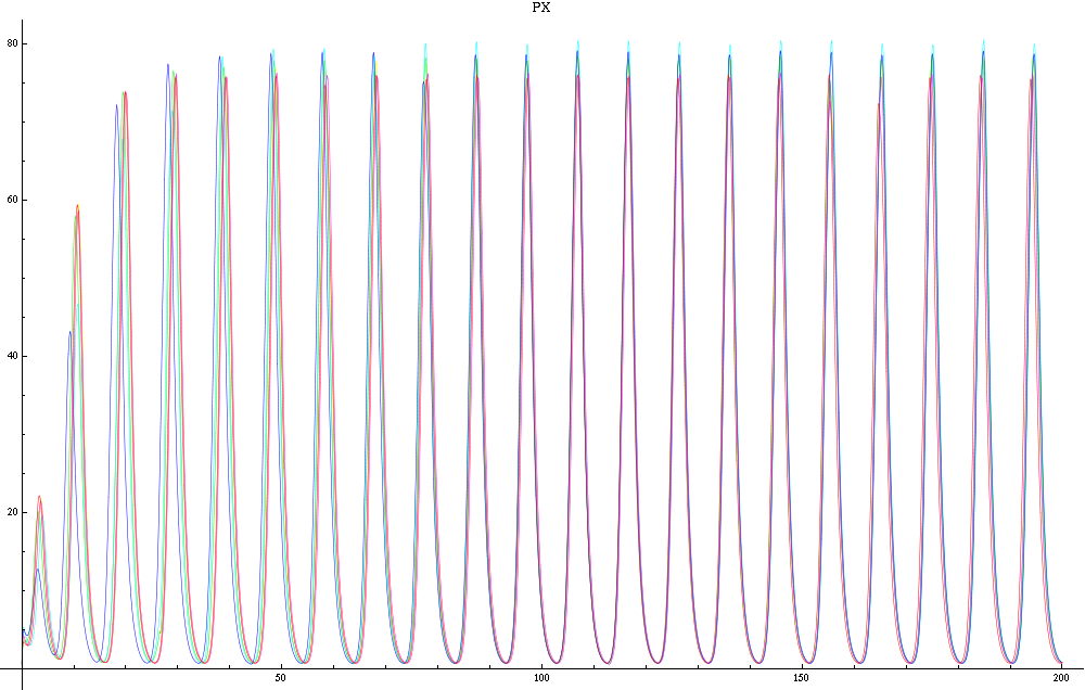
| + | Image:C-px21.png|Figure 2a: Simulation using Mathematica of the Repressilator Network. The plot shows the concentration of AI against time (in arbitrary units). Similar to configuration as fig. 1, but the clusters are closer (distance ~1). | ||
| + | Image:C-px30.png|Figure 2b: Similar to fig. 2a, but with a different distance between the clusters. Same configuration as fig. 1 (distance ~10). | ||
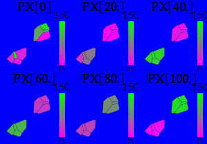
| + | Image:C-px.gif|Figure 2c: Movie showing the spatial distribution of the concentration of AI as time goes forward. Same configuration as fig. 1. | ||
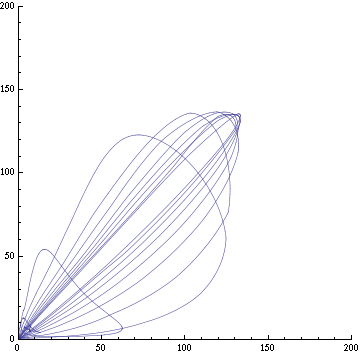
| + | Image:C-parametric-px1px3.png|Figure 3a: The concentration of AI of two cells in different clusters against each other. Same configuration as fig. 1. | ||
| + | Image:C-parametric-x1px1.png|Figure 3b: The concentration of X and AI in a given cell. Same configuration as fig. 1. | ||
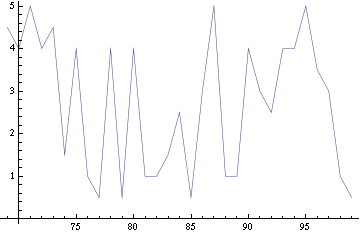
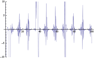
| + | Image:C-errorEx.png|Figure 4: Checking the compatibility of the solution (of the fig. 1, 2b and 3) with the equations. Ideally, the graph would be identically zero -- meaning that the solution agrees everywhere with the equations. | ||
| + | </gallery> | ||
| + | |||
| + | ===Future Development=== | ||
| + | |||
| + | Eventually, if everything goes smoothly of course, we will use more realistic rates for the various reactions: some might be found in the literature (for instance, in [2,3]), others will be experimentally measured. If the processing power is not too high, we will aim at increasing the number of cells and clusters to something more spectacular (>100 and >4 respectively). We are also interested in playing with how xCellerator handles connection between cells to allow the clusters to remain in contact when looking at large distance (>35). Currently, the clusters can become disjoint when the Bounded Cell Voronoi graphs shows a rupture (although, not always, as we are using Delaunay Triangulation as implemented in xCellerator). Furthermore, we will attempt to do a parameter analysis over the various rates, so that we will try to find the critical values for which peculiar behaviour happens in the system of clusters. Indeed, there might exist some specific values of rates or other parameters for which the system is damped for example. An interesting venue would be to model the diffusion in a different way than by a rate; however, that would probably require to use a non-xCellerator continuous model with the diffusion equation replacing the current external equation. | ||
| + | |||
| + | ===References=== | ||
| + | |||
| + | [1] xCellerator: http://xlr8r.info/ | ||
| + | |||
| + | [2] Jordi Garcia-Ojalvo, Michael B. Elowitz, and Steven H. Strogatz. Modeling a synthetic multicellular clock: Repressilators coupled by quorum sensing, PNAS vol. 101 no. 30, 2004. | ||
| + | |||
| + | [3] Michael B. Elowitz and Stanislas Leibler. A synthetic oscillatory network of transcriptional regulators. Nature, vol. 403, 2000. | ||
| + | |||
| + | ===Annexe 1=== | ||
| + | |||
| + | <gallery> | ||
| + | Image:C-px19.png|Concentration of AI against time (arbitrary units). The clusters have a distance ~1. | ||
| + | Image:C-px20.png|Concentration of AI against time (arbitrary units). The clusters have a distance ~2. | ||
| + | Image:C-px21.png|Concentration of AI against time (arbitrary units). The clusters have a distance ~3. | ||
| + | Image:C-px22.png|Concentration of AI against time (arbitrary units). The clusters have a distance ~4. | ||
| + | Image:C-px23.png|Concentration of AI against time (arbitrary units). The clusters have a distance ~5. | ||
| + | Image:C-px24.png|Concentration of AI against time (arbitrary units). The clusters have a distance ~6. | ||
| + | Image:C-px25.png|Concentration of AI against time (arbitrary units). The clusters have a distance ~7. | ||
| + | Image:C-px26.png|Concentration of AI against time (arbitrary units). The clusters have a distance ~8. | ||
| + | Image:C-px27.png|Concentration of AI against time (arbitrary units). The clusters have a distance ~9. | ||
| + | Image:C-px28.png|Concentration of AI against time (arbitrary units). The clusters have a distance ~10. | ||
| + | Image:C-px29.png|Concentration of AI against time (arbitrary units). The clusters have a distance ~11. | ||
| + | Image:C-px30.png|Concentration of AI against time (arbitrary units). The clusters have a distance ~12. | ||
| + | Image:C-px31.png|Concentration of AI against time (arbitrary units). The clusters have a distance ~13. | ||
| + | Image:C-px32.png|Concentration of AI against time (arbitrary units). The clusters have a distance ~14. | ||
| + | Image:C-px33.png|Concentration of AI against time (arbitrary units). The clusters have a distance ~15. | ||
| + | Image:C-px34.png|Concentration of AI against time (arbitrary units). The clusters have a distance ~16. | ||
| + | Image:C-px35.png|Concentration of AI against time (arbitrary units). The clusters have a distance ~17. | ||
| + | Image:C-px36.png|Concentration of AI against time (arbitrary units). The clusters have a distance ~18. | ||
| + | Image:C-px37.png|Concentration of AI against time (arbitrary units). The clusters have a distance ~19. | ||
| + | Image:C-px38.png|Concentration of AI against time (arbitrary units). The clusters have a distance ~20. | ||
| + | Image:C-px39.png|Concentration of AI against time (arbitrary units). The clusters have a distance ~21. | ||
| + | </gallery> | ||
| + | |||
| + | ===Annexe 2=== | ||
| + | |||
| + | The set of equations changed since these graphs here have been generated, but more results are available and, so, the graphs will be left here for now. This code takes about 5 minutes to run for a small configuration (2 clusters of 2 cells each). | ||
| + | |||
| + | For a given distance between the two clusters of cells (fig. 1), we plot the concentration of AI in each cells versus time (fig. 2). From there, we extract two informations: synchronization time and phase difference (fig. 4-5). The two clusters are actually not distinguishable for distances below 20 (fig. 4-5). The general trend in fig. 4 seems to be that the longer the distance, the longer it takes to synchronize, but we also noticed that after a certain distance, the two clusters are no longer in synchrony. Unless they just take much longer to synchronize than the windows of the graph -- in which case we would need to run the simulation for a longer time to observe synchronization. As for the graph of the phase difference (fig. 5) made to different scales, we have yet to figure out what could be the pattern. The results are also presented in the form of parametric plots involving the concentration of AI (fig. 3) and some short movies can be generated to show the spatial distribution of the concentration of AI as time moves forward (fig. 2c). An interesting point we noticed up to now is that, whatever the initial conditions, the system of cells has an oscillatory behaviour as in fig. 2. | ||
| + | |||
| + | <gallery> | ||
| + | Image:visualisation.png|Figure 1a: This is a Bounded Cell Voronoi graph representing the cells in the model. It participates in the determination of the nearest neighbour cells. However, the cells are represented internally by points as in fig. 1b. | ||
| + | Image:Visualisation-dot.png|Figure 1b: The cells are represented in the model as circular points of radius w. | ||
Image:px.png|Figure 2a: Simulation using Mathematica of the Repressilator Network with four cells shown in fig. 1. The plot shows the concentration of AI against time (in arbitrary units). | Image:px.png|Figure 2a: Simulation using Mathematica of the Repressilator Network with four cells shown in fig. 1. The plot shows the concentration of AI against time (in arbitrary units). | ||
Image:Px27.png|Figure 2b: Similar to fig. 2a, but with a different distance between the clusters. | Image:Px27.png|Figure 2b: Similar to fig. 2a, but with a different distance between the clusters. | ||
| Line 66: | Line 118: | ||
Image:ErrorEx.png|Figure 6: Checking the compatibility of the solution with the equations. Ideally, the graph would be identically zero -- meaning that the solution agrees everywhere with the equations. | Image:ErrorEx.png|Figure 6: Checking the compatibility of the solution with the equations. Ideally, the graph would be identically zero -- meaning that the solution agrees everywhere with the equations. | ||
</gallery> | </gallery> | ||
| - | |||
| - | |||
| - | |||
| - | |||
| - | |||
| - | |||
| - | |||
Latest revision as of 17:50, 9 August 2008
| Home | The Team | The Project | Parts | Notebook | Modeling | Links | Sponsors |
|---|
Contents |
Background
Using coupled differential equations, we are modeling the Repressilator network, which is a composed of three genes, whose product proteins are repressing each other's growth. This cycle is taking place in each of a colony of cells, who communicate amongst themselves by exchanging an autoinducer molecule (AI, or PX here). The model attempts to take into account a sparse, heterogeneous distribution of many cells (grouped in clusters) with depletion of the autoinducer molecule and leakage while assuming continuous levels of the different proteins, as well as a continuous spatial distribution of these proteins.
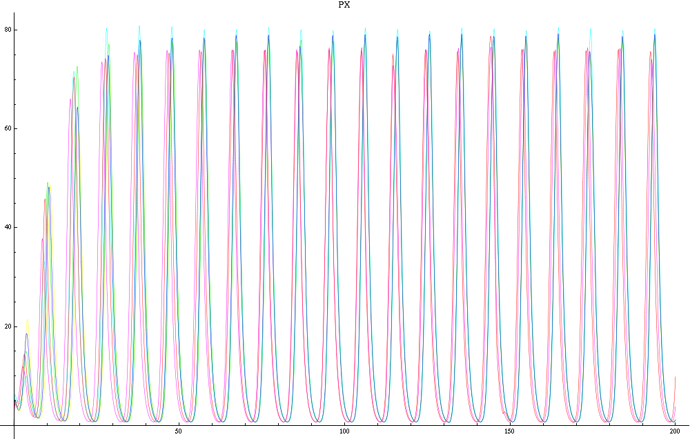
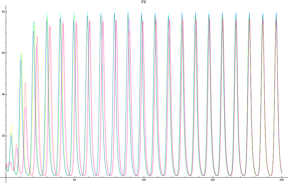
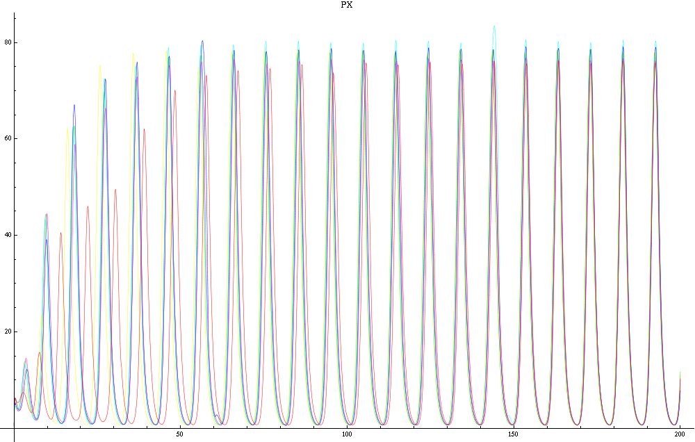
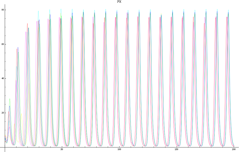
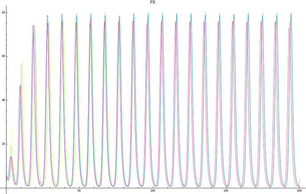
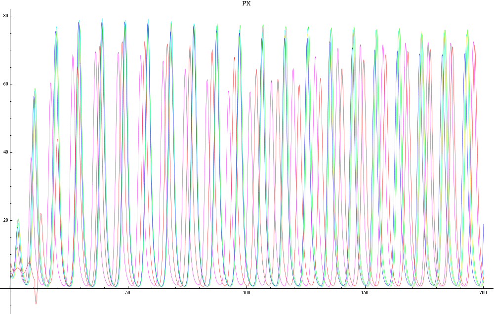
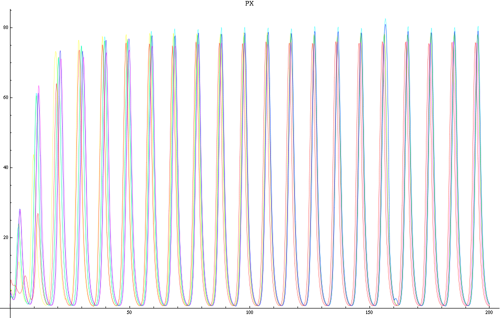
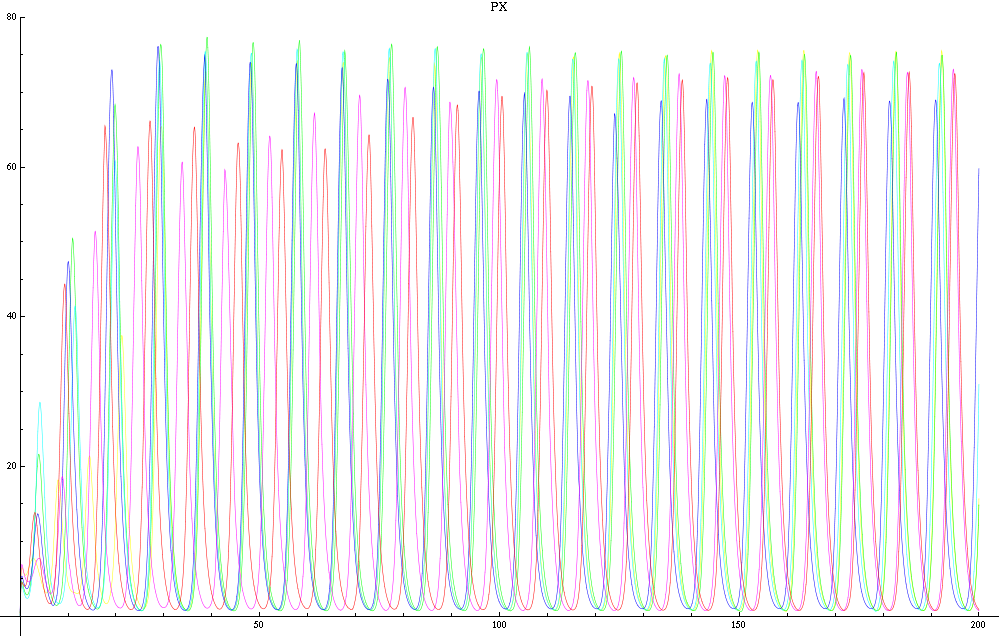
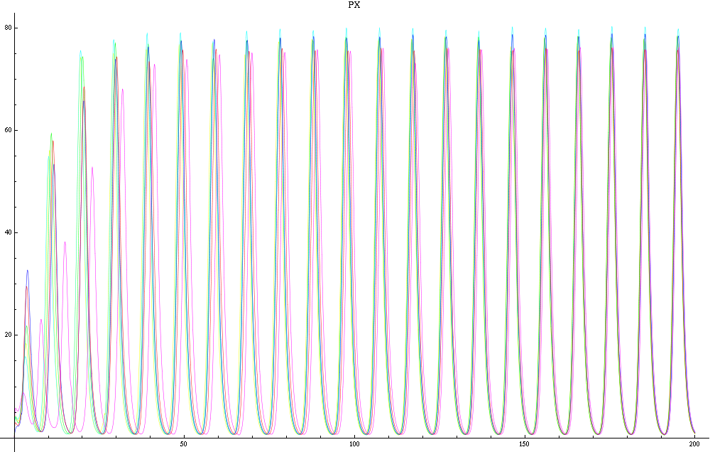
For this purpose, the model is currently being coded up in Mathematica. The simulations, based on that continuous model, are generated using xCellerator [1] and NDelayDSolve for different cell configurations (fig. 1); the results obtained are graphs of the concentration of molecules in the system versus time (fig. 2). That is, our interest lies in understanding the behaviour of the clusters with respect to each other (for instance, the phase difference or the synchronization time as in fig. 4-5). As of now, a low number (~4) of cells in two clusters is being used for testing, but a higher one (>100) in more clusters will be reached later.
The Model
For the interested reader, the system of differential equations for the Repressillator network is composed of internal and external reaction. X, Y and Z are mRNA's and PX, PY and PZ their respectively associated product proteins. AI is assumed to be the same as PX. The internal reactions model what happens inside a cell and the equations are
PYi'(t) = -βPYi(t) + βYi(t)
PZi'(t) = -βPZi(t) + βZi(t)
 Xi'(t) = α0 + [α + α1PZin(t)]/[Kn + PZin(t)] - k1Xi(t)
 Yi'(t) = α0 + [α + α1PXin(t)]/[Kn + PXin(t)] - k1Yi(t)
 Zi'(t) = α0 + [α + α1PYin(t)]/[Kn + PYin(t)] - k1Zi(t).
The external reaction models the interaction between the cells:
PXi'(t) = -βPXi(t) + βXi - γPXi(t) + ΣjwγPXj(t-τij)/[2Piτijv].
On the right hand side, the first term models decaying of AI, the second the creation of AI from X and the third the diffusion of AI in the network. The variables τij = distij/v and α0, α1, α, β, k1, v and w are parameters; distij is the distance between cells i and j. Some values were taken from [2,3]. The index i runs over all the cells in the system; the sum over j runs over nearest neighbour cells. Nearest neighbour cells are determined by the Bounded Cell Voronoi diagram with Delaunay Triangulation by xCellerator. Quoting [2], β is the ratio between the mRNA and protein parameter lifetimes, and the mRNA concentrations have been rescaled by their translation efficiency (proteins produced per mRNA, assumed equal for the three genes).
Here's the reasoning behind the external equation. The proportion of autoinducer (AI, or PX here) molecules from cell i reaching cell j is p=w/[distij2Pi], which is the width of a cell (the target cell) over the circumference of a circle of radius distij. The number of AI molecules reaching the target cell is therefore the quantity emitted PXi times that proportion. However, we need to evaluate PXi at a previous time, since the AI moves slowly. Indeed, the time the molecules will take to diffuse from cell i to j is τij. The rate at which AI molecules go out of the cells is γ which we assume is proportional to the rate of creation of AI, β. Hence, the rate of AI molecules leaving cell i is n=γPXi(t-τij). Therefore, the rate of change of the AI molecule due to diffusion is the product of the proportion reaching cell j and the number of AI emitted; in other words,
np = -βPXi(t-τij)w/[distij2Pi]
   = -wγPXi(t-τij)/[2Piτijv].
Now, we sum over all nearest over all nearest neighbours of i. And we are done.
Journal
The Mathematica notebook used to model the repressillator uses xCellerator to create the differential equations representing the chemical reactions involved. This original version of the notebook is able to deal with randomly distributed close-packed configuration of cells and predicts near-perfect synchronization of the cells in a relatively short time. In this version, the system of differential equations was solved using NDSolve, a standard numerical solver in Mathematica -- which is, however, unable to deal with delay equations. Hence, the equations were not evaluated at retarded times at first. Indeed, our first approach was to add null cells in the network in order to delay the diffusion of molecules. The nulls cells, or pseudo cells, are just grid point where no internal cell reaction occurs, but only diffusion to the next grid point. However, the results such as phase difference depended too heavily on the number of such null cells. The general oscillating behaviour seemed correct though. As we did not have a mean of estimating a realistic distribution of such null cells, they did not seem reliable enough. Furthermore, they were taking similar computing time as of interesting/standard cells -- eating away the computational resources available.
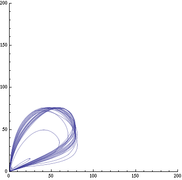
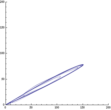
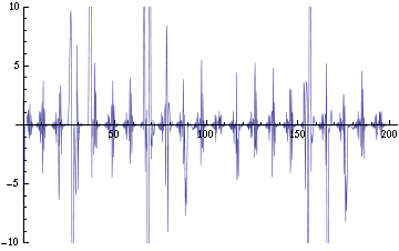
We are now replacing NDSolve with NDelayDSolve to solve the system and we are therefore able to evaluated our equations at retarded times. We are not using null cells anymore. The value of the delays corresponds to the time the molecules of AI diffuse the intercellular distance: the reasoning being that each cells effectively "sees" the concentration of another cell at an earlier time -- the time the molecules take to diffuse between them. We have one worry for now with using NDelayDSolve rather than NDSolve: Mathematica warns that it is not able to reach the prescribed accuracy/precision during the computation. When checking the compatibility of the solution found with the equations, we find "reasonable" errors most of the time, but periodic (roughly at the same time as the peaks as seen in fig. 2) sudden kicks to high discrepancies (fig. 4). We changed the numerical methods used to solve the delay equations in order to minimize the error profile seen in fig. 4: we currently use Stiffness Switching with Explicit and Linearly Implicit Euler. The code as it is takes about 15 minutes to run for a small configuration (2 clusters of 2 and 4 cells). We are still trying to understand how xCellerator handles consistently the indices in the external equations.
For a given distance between the two clusters of cells (fig. 1), we plot the concentration of AI in each cells versus time (fig. 2 and Annexe 1). The results are also presented in the form of parametric plots involving the concentration of AI (fig. 3) and some short movies can be generated to show the spatial distribution of the concentration of AI as time moves forward (fig. 2c). An interesting point we noticed up to now is that, whatever the initial conditions, the system of cells has an oscillatory behaviour as in fig. 2. Since the equations have been modified recently, patterns related to phase difference and synchronization time have yet to be figured out.
Future Development
Eventually, if everything goes smoothly of course, we will use more realistic rates for the various reactions: some might be found in the literature (for instance, in [2,3]), others will be experimentally measured. If the processing power is not too high, we will aim at increasing the number of cells and clusters to something more spectacular (>100 and >4 respectively). We are also interested in playing with how xCellerator handles connection between cells to allow the clusters to remain in contact when looking at large distance (>35). Currently, the clusters can become disjoint when the Bounded Cell Voronoi graphs shows a rupture (although, not always, as we are using Delaunay Triangulation as implemented in xCellerator). Furthermore, we will attempt to do a parameter analysis over the various rates, so that we will try to find the critical values for which peculiar behaviour happens in the system of clusters. Indeed, there might exist some specific values of rates or other parameters for which the system is damped for example. An interesting venue would be to model the diffusion in a different way than by a rate; however, that would probably require to use a non-xCellerator continuous model with the diffusion equation replacing the current external equation.
References
[1] xCellerator: http://xlr8r.info/
[2] Jordi Garcia-Ojalvo, Michael B. Elowitz, and Steven H. Strogatz. Modeling a synthetic multicellular clock: Repressilators coupled by quorum sensing, PNAS vol. 101 no. 30, 2004.
[3] Michael B. Elowitz and Stanislas Leibler. A synthetic oscillatory network of transcriptional regulators. Nature, vol. 403, 2000.
Annexe 1
Annexe 2
The set of equations changed since these graphs here have been generated, but more results are available and, so, the graphs will be left here for now. This code takes about 5 minutes to run for a small configuration (2 clusters of 2 cells each).
For a given distance between the two clusters of cells (fig. 1), we plot the concentration of AI in each cells versus time (fig. 2). From there, we extract two informations: synchronization time and phase difference (fig. 4-5). The two clusters are actually not distinguishable for distances below 20 (fig. 4-5). The general trend in fig. 4 seems to be that the longer the distance, the longer it takes to synchronize, but we also noticed that after a certain distance, the two clusters are no longer in synchrony. Unless they just take much longer to synchronize than the windows of the graph -- in which case we would need to run the simulation for a longer time to observe synchronization. As for the graph of the phase difference (fig. 5) made to different scales, we have yet to figure out what could be the pattern. The results are also presented in the form of parametric plots involving the concentration of AI (fig. 3) and some short movies can be generated to show the spatial distribution of the concentration of AI as time moves forward (fig. 2c). An interesting point we noticed up to now is that, whatever the initial conditions, the system of cells has an oscillatory behaviour as in fig. 2.
 "
"


