Team:KULeuven/Model/Filter
From 2008.igem.org
m (→ODE's) |
m |
||
| (9 intermediate revisions not shown) | |||
| Line 1: | Line 1: | ||
| + | {{:Team:KULeuven/Tools/Styling}} | ||
| + | {{:Team:KULeuven/Tools/Scripting}} | ||
{{:Team:KULeuven/Tools/Header}} | {{:Team:KULeuven/Tools/Header}} | ||
| - | + | [[Image:pictogram_filter.png|120px|right]] | |
== Filter == | == Filter == | ||
| Line 129: | Line 131: | ||
[[Image:Sim_filter_1.png|800px|center|filter]] | [[Image:Sim_filter_1.png|800px|center|filter]] | ||
| - | |||
| - | |||
====1. AND gate of the filter==== | ====1. AND gate of the filter==== | ||
In the simulation we can clearly see this series of events: | In the simulation we can clearly see this series of events: | ||
| + | [[Image:Filter 1.PNG|right]] | ||
* when dark blue(ribokey) starts to increase, red (T7) also starts to increase, giving rise to an increasing amount of lactonase (blue) = AND-GATE. | * when dark blue(ribokey) starts to increase, red (T7) also starts to increase, giving rise to an increasing amount of lactonase (blue) = AND-GATE. | ||
* when dark blue(ribokey) starts to decrease, red (T7) also starts to decrease, but much slower. The lactonase also starts to decrease, as it should be. | * when dark blue(ribokey) starts to decrease, red (T7) also starts to decrease, but much slower. The lactonase also starts to decrease, as it should be. | ||
| Line 172: | Line 173: | ||
Another way to see the filtering effect is to look at the ratio of GFP to Lactonase. This figure clearly shows the disproportionality between GFP and lactonase for the pulses shorter than 1000 seconds. The best filtering effect occurs for pulses around 100 seconds. This figure also shows that placing the filter in front of a signal wil lower this signal with a factor of at least 25 (full throughput in the filter). This base factor should be multiplied by ~8 for pules around 100 seconds. This is the filtering effect quantitated: pulses of only 100 seconds will produce almost 25 * 8 = 200 times more GFP than Lactonase. A factor 25 characteristic of the system and a variable extra filtering factor that is a function of pulse length and is maximal (8) for pulses of 100 seconds. | Another way to see the filtering effect is to look at the ratio of GFP to Lactonase. This figure clearly shows the disproportionality between GFP and lactonase for the pulses shorter than 1000 seconds. The best filtering effect occurs for pulses around 100 seconds. This figure also shows that placing the filter in front of a signal wil lower this signal with a factor of at least 25 (full throughput in the filter). This base factor should be multiplied by ~8 for pules around 100 seconds. This is the filtering effect quantitated: pulses of only 100 seconds will produce almost 25 * 8 = 200 times more GFP than Lactonase. A factor 25 characteristic of the system and a variable extra filtering factor that is a function of pulse length and is maximal (8) for pulses of 100 seconds. | ||
| - | + | ||
| + | <html> | ||
| + | <div class="center"> | ||
| + | <div class="noborder" style="overflow: auto; width: 900px; height: 370px;"> | ||
| + | <div class="noborder" style="width: 850px;"> | ||
| + | <img src="https://static.igem.org/mediawiki/2008/0/0c/GFP_Lactonase.png" style="float: left; width: 400px; height: 350px; margin: 0 5px;" /> | ||
| + | <img src="https://static.igem.org/mediawiki/2008/1/13/GFP_lactonase_norm.png" style="float: left; width: 400px; height: 350px; margin: 0 5px;" /> | ||
| + | </div></div></div></html> | ||
| + | |||
| + | <br> | ||
| + | |||
| + | Another nice way to visualazise the same filtering effect can be seen in the following figures. In the left figure, 4 input pulses are given in sequence. The first lasts 100 seconds, the second 500, the third 2500 while the last one remains indefinateley. | ||
| + | The maximal output (result of the 4th pulse), both non-filtered and filtered are set to 1, normalizing the signals. It is now very easy to see the filtering in effect on the zoomed-in right figure and the ratio's can be compared with the y-values of the previous figure. | ||
| + | |||
| + | <html> | ||
| + | <div class="center"> | ||
| + | <div class="noborder" style="overflow: auto; width: 900px; height: 320px;"> | ||
| + | <div class="noborder" style="width: 900px;"> | ||
| + | <img src="https://static.igem.org/mediawiki/2008/1/18/Filter_extra.png" style="float: left; width: 440px; height: 300px; margin: 0 5px;" /> | ||
| + | <img src="https://static.igem.org/mediawiki/2008/0/0b/Filter_extra_zoom.png" style="float: left; width: 440px; height: 300px; margin: 0 5px;" /> | ||
| + | </div></div></div></html> | ||
| + | |||
| + | <br> | ||
=== References === | === References === | ||
Latest revision as of 23:12, 29 October 2008
Contents |
Filter
Position in the system
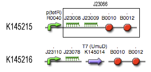
The filter is positioned immediately after the input, because its job is to filter out possible noise signals or background signals that aren't caused by the "desease". It is the starting piece of the whole system, situated before the invertimer- and the reset-subsystem.
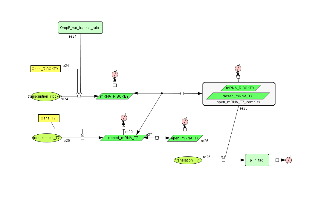
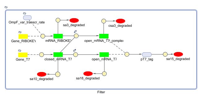
Describing the system
see also: Project:Filter
ODE's
Parameters
| Name | Value | Comments | Reference |
|---|---|---|---|
| Degradation rates | |||
| dpT7 tag | 0.00155 s-1 | UmuD tag added to speed up degradation of otherwise too stable T7 polymerase | [4] [5] [8] |
| dmRNA RIBOKEY | 0.00462 s-1 | estimate: because this RNA isn't translated, it degrades faster | [3] |
| dclosed mRNA T7 | 0.00462 s-1 | estimate: because this mRNA isn't translated, it degrades faster | [3] |
| dopen mRNA T7 | 0.00231 s-1 | [3] | |
| dopen mRNA T7 complex | 0.00231 s-1 | [3] | |
| Equilibrium constants | |||
| Keq 1 | 0,015 [M] | between closed and open T7 mRNA, models competition, experimental | [1] [2] |
| Keq 2 | 0.0212 [M] | between closed T7 mRNA and key unlocked mRNA complex, models competition, experimental | [1] [2] |
| Rate constants | |||
| kdis | 0.00416 s-1 | estimate derived from experimental values | [1] |
| kcomplex | 0.00237 s-1 | estimate derived from experimental values | [1] |
| kclosed | 500 s-1 | estimate derived from experimental values | [1] |
| kopen | 7.5 s-1 | estimate derived from experimental values | [1] |
| ktranslation | 0.167 s-1 | estimate: lock defined translation rate for T7 RNA pol | [7] |
| Transcription rates | |||
| TetR_var_transcr_rate | p(TetR) dependent | (RiboKey) between 5E-5 and 0.0125 s-1 ~ [aTc] | [6] |
| kmRNA T7 | 0,0011 s-1 | weak constitutive promoter J23109 | [7] |
Remark: The key-lock system has been enhanced to 0.3%-14% (new parameters have been added)
Models
CellDesigner (SBML file)
Matlab (SBML file)
Simulations
1. AND gate of the filter
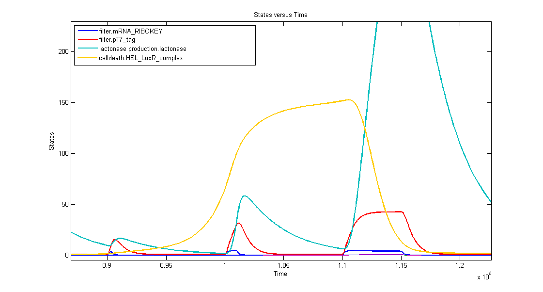
In the simulation we can clearly see this series of events:
- when dark blue(ribokey) starts to increase, red (T7) also starts to increase, giving rise to an increasing amount of lactonase (blue) = AND-GATE.
- when dark blue(ribokey) starts to decrease, red (T7) also starts to decrease, but much slower. The lactonase also starts to decrease, as it should be.
The short lifetime of the ribokey compared to the lifetime of the T7-protein, guarantees that the AND-GATE always works perfectly fine: when there's no more input, the ribokey will rapidly decrease (and disappear) and makes sure that the AND-GATE is not activated anymore, even when the T7-protein is slowly decreasing.
2. Filtering in practice
In the simulation three kinds of inputpulses have been used:
- First pulse: 300s
- small peak of lactonase
- no influence on the timer
- Second pulse: 1000s
- medium peak of lactonase
- influences the timer by levelling the timing capabilities, but it doesn't reset the timer
- Third pulse: 5000s
- huge peak of lactonase
- reset of the timer: amount of complex goes to zero
3. Proof of filtering capacities
As proof of the filtering capacities, we'll compare the maximum amount of GFP with the maximum amount of Lactonase as a function of the pulse length of TetR. We've chosen Lactonase and GFP because they differ only in the absence or presence of the filter, all other parameters are identical (eg. degradation rate). The model used here consists only of the filter, the output and the lactonase productions subsystems.
The left figures shows us a clear difference between the amount of GFP and lactonase for almost every pulse length. The explanation for the (almost constant) big difference for pulses longer than 1000 seconds is the following. For such long pulses, the filter can be considered as fully active, such that the only differences between the output and the lactonase production are characteristics of the ribokey/lock and the difference in transcription rates between E. coli's RNA polymerase II and phage T7's polymerase. For a pulse shorter than 1000 seconds the filter is not fully active. This creates a filtering effect. If we just look at the first 1000 seconds (right figures), we see that the amount of Lactonase remains more or less the same while the amount of GFP increases very fast.


Another way to see the filtering effect is to look at the ratio of GFP to Lactonase. This figure clearly shows the disproportionality between GFP and lactonase for the pulses shorter than 1000 seconds. The best filtering effect occurs for pulses around 100 seconds. This figure also shows that placing the filter in front of a signal wil lower this signal with a factor of at least 25 (full throughput in the filter). This base factor should be multiplied by ~8 for pules around 100 seconds. This is the filtering effect quantitated: pulses of only 100 seconds will produce almost 25 * 8 = 200 times more GFP than Lactonase. A factor 25 characteristic of the system and a variable extra filtering factor that is a function of pulse length and is maximal (8) for pulses of 100 seconds.


Another nice way to visualazise the same filtering effect can be seen in the following figures. In the left figure, 4 input pulses are given in sequence. The first lasts 100 seconds, the second 500, the third 2500 while the last one remains indefinateley. The maximal output (result of the 4th pulse), both non-filtered and filtered are set to 1, normalizing the signals. It is now very easy to see the filtering in effect on the zoomed-in right figure and the ratio's can be compared with the y-values of the previous figure.


References
| [1] | “Berkeley2006-RiboregulatorsMain - IGEM”; http://parts2.mit.edu/wiki/index.php/Berkeley2006-RiboregulatorsMain. |
| [2] | F.J. Isaacs et al., “Engineered riboregulators enable post-transcriptional control of gene expression,” Nat Biotech, vol. 22, Jul. 2004, pp. 841-847. |
| [3] | J.A. Bernstein et al., “Global analysis of mRNA decay and abundance in Escherichia coli at single-gene resolution using two-color fluorescent DNA microarrays,” Proceedings of the National Academy of Sciences of the United States of America, vol. 99, Jul. 2002, pp. 9697–9702. |
| [4] | “IGEM:Tsinghua/2007/Projects/RAP - OpenWetWare”; http://www.openwetware.org/wiki/IGEM:Tsinghua/2007/Projects/RAP#Model_and_simulation. |
| [5] | M. Gonzalez et al., “Lon-mediated proteolysis of the Escherichia coli UmuD mutagenesis protein: in vitro degradation and identification of residues required for proteolysis,” Genes Dev., vol. 12, Dec. 1998, pp. 3889-3899. |
| [6] | M. Bon, S.J. McGowan, and P.R. Cook, “Many expressed genes in bacteria and yeast are transcribed only once per cell cycle,” FASEB J., vol. 20, Aug. 2006, pp. 1721-1723. |
| [7] | “Part:BBa J23109 - partsregistry.org”; http://partsregistry.org/Part:BBa_J23109. |
| [8] | J.P. McDonald et al., “Regulation of UmuD cleavage: role of the amino-terminal tail,” Journal of Molecular Biology, vol. 282, Oct. 1998, pp. 721-730. |
 "
"


