Team:Paris/Modeling/BOB/Akaike
From 2008.igem.org
| (5 intermediate revisions not shown) | |||
| Line 1: | Line 1: | ||
| - | {{Paris/ | + | {{:Team:Paris/MenuBackup}} |
<br> | <br> | ||
| - | <center><html><div style="color:#275D96; font-size:2em;">Depending on the experimental constraints, how can we be helped by <br>mathematical criterions ?</div></html></center> | + | <center><html><div style="color:#275D96; font-size:2em;">Depending on the experimental constraints, how can we be helped by <br><br>mathematical criterions ?</div></html></center> |
<br> | <br> | ||
| - | * When building a model, it is of the utmost importance to present a justification of the choice made along the transposition process from biological reality to mathematical representation. The aim of this section is to introduce a mathematical justification of our choices in the [[Team:Paris/Modeling/BOB|BOB approach]] since it seems remote from biological | + | * When building a model, it is of the utmost importance to present a justification of the choice made along the transposition process from biological reality to mathematical representation. The aim of this section is to introduce a mathematical justification of our choices in the [[Team:Paris/Modeling/BOB|BOB approach]] since it seems remote from biological reality compared to our [[Team:Paris/Modeling/hill_approach|APE approach]]. The criterion presented below are to help choosing the most reluctant model '''given the experimental constraints'''. |
<br> | <br> | ||
= Short introduction to the criteria = | = Short introduction to the criteria = | ||
Latest revision as of 07:06, 30 October 2008
Go back to the normal Wiki
mathematical criterions ?
- When building a model, it is of the utmost importance to present a justification of the choice made along the transposition process from biological reality to mathematical representation. The aim of this section is to introduce a mathematical justification of our choices in the BOB approach since it seems remote from biological reality compared to our APE approach. The criterion presented below are to help choosing the most reluctant model given the experimental constraints.
Short introduction to the criteria
- Using linear equations in a biological system might seem awkards. However, we wanted to check the relevance of this approach. We have been looking for a criterium that would penalize a system that had many parameters, but that would also penalize a system which quadratic error would be too important while fitting experimental values. The goal here is to decide whether, assuming that the experimental data looks like a model based on Hill functions, the linear part of the BOB model is obsolete or not.
- Akaike and Schwarz criteria taken from the information theory met our demands quite well :
where n denotes the number of experimental values, k the number of parameters and RSS the residual sum of squares. The best fitting model is the one for which those criteria are minimized.
- It is remarquable that Akaike criterion and Hurvich and Tsai criterion are alike. AICc is therefore used for small sample size, but converges to AIC as n gets large. Since we will work with 20 points for each experiment, it seemed relevant to present both models. In addition, Schwarz criterion is meant to be more penalizing.
Experiment
- As an experiment, we wished to compare the two models presented below :
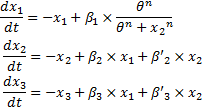
System#1 : using the linear equations from our BOB approach :
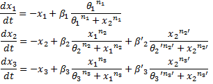
System#2 : using classical Hill functions :
- We made a set of data out of a noised Hill function. In fact, our data set was made by using the same equations as System#2, but we introduced a normal noise for each point. Thus, System#1 is penalized because its RSS will be greater than that of System#2. Nevertheless, System#2 will be more penalized by its number of parameters.
- With Matlab, we run a fitting simulation for each system, and we obtained the RSS. We then evaluated the different criteria for both models. We chose to act as if the length of our experimental data set was 20 (which is what we would have gotten in reality). The results are presented below.
| Comparison of the systems for n=20 | ||
|---|---|---|
| Criteria | System#1 | System#2 |
| AIC | 26.7654 | 32.0035 |
| AICc | 38.7654 | 168.0035 |
| BIC | 22.9435 | 24.3596 |
| Comparison of the systems for n=100 | ||
|---|---|---|
| Criteria | System#1 | System#2 |
| AIC | 169.5495 | 32.1150 |
| AICc | 171.1147 | 38.5912 |
| BIC | 172.0100 | 37.0360 |
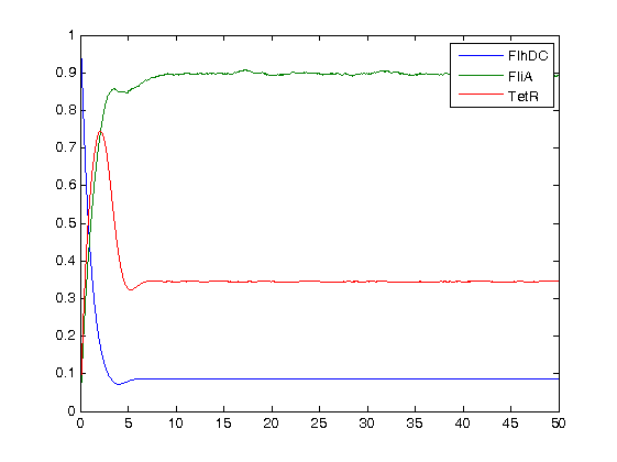
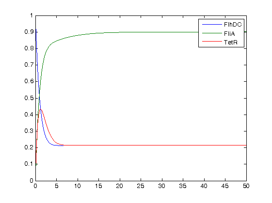
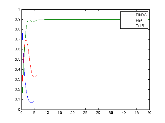
- Finally, we wanted to check that those numerical simulation did not hide anything. Then, we run the simulation plots obtained for the parameters that best fitted. Here are the results :
Then, we see that the Bob model does not fit that well, but under certain conditions it is not so bad. Indeed, if the data set is short, Bob model can be used as a reluctant model, that helps understanding the dynamics.
- Consequently, what have we proved? These results show that:
- Firstly, we may see that the AICc does converge to AIC for greater values of n.
- Then, we may see that, as predicted, System#2 is not penalized anymore for greater values of n, although System#1 is. Consequently, we may adapt our system knowing the length of the data set we are going to obtain experimentally.
- Furthermore, since the use of more parameters is quite penalizing for a small set of data, and since the criteria are minimized for System#1, the first subsystem of our BOB model is not irrelevant.
- However, since for a larger set of data System#2 minimizes the criteria, these criteria cannot decide whether a model is "better" than another one, since those criteria are arbitrary. Yet, they may help us find a better compromise between simplification and accuracy.
- One must be careful when building a model, since chosing the number of parameters and deciding how deep one wishes to go into detail, influences the goal and the results of a model. It is therefore important to understand that a model has to be conceived to achieve a precise aim.
- Then, it is always useful to use different models, knowing that each model meets a certain demand. Here, our full model (APE) will be used to present a highly detailed overview of the processes that take place in the system. In the mean time, the BOB approach is a reasonable mean to explore the system quickly and understand its ins and outs.
A fundamental tool?
Why can we introduce this seemingly awkard criteria as being a fundamental tool? This precise criteria enables the mathematician to adapt its model. In fact, in that respect, conducting this analysis over his model gives tangible arguments to the mathematician to use such and such model. Indeed, for example in our precise case, if we have about 20 experimental points to fit, BOB approach is sufficient. However, if we get 50 points, BOB approach would be inadequate compared to APE. We believe that this kind of criteria is an essential tool, that might help the model maker to comprehend and control the assumptions he made while creating his model.
- We mostly used the definition of the criteria given in :
[http://www.liebertonline.com/doi/pdf/10.1089/rej.2006.9.324 K. Kikkawa.Statistical issue of regression analysis on development of an age predictive equation. Rejuvenation research, Volume 9, n°2, 2006.]
- Here can be found the programs used in this section.
 "
"
