Team:Paris/Modeling/BOB/Akaike
From 2008.igem.org
(→A fundamental tool?) |
(→Experiment) |
||
| Line 22: | Line 22: | ||
[[Image:syste_akaike_2_bis.jpg|center]]<br> | [[Image:syste_akaike_2_bis.jpg|center]]<br> | ||
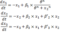
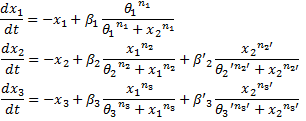
* We made a set of data out of a noised Hill function. In fact, our data set was made by using the same equations as System#2, but we introduced a normal noise for each point. Thus, System#1 is penalized because its RSS will be greater than that of System#2. Nevertheless, System#2 will be more penalized by its number of parameters. | * We made a set of data out of a noised Hill function. In fact, our data set was made by using the same equations as System#2, but we introduced a normal noise for each point. Thus, System#1 is penalized because its RSS will be greater than that of System#2. Nevertheless, System#2 will be more penalized by its number of parameters. | ||
| - | * With Matlab, we run a fitting simulation for each system, and we obtained the RSS. We then evaluated the different criteria for both models. The results are presented below. | + | * With Matlab, we run a fitting simulation for each system, and we obtained the RSS. We then evaluated the different criteria for both models. We chose to act as if the length of our experimental data set was 20 (which is what we would have gotten in reality). The results are presented below. |
<center> | <center> | ||
{| | {| | ||
| Line 73: | Line 73: | ||
* Consequently, what have we proved? These results show that: | * Consequently, what have we proved? These results show that: | ||
** Firstly, we may see that the AICc does converge to AIC for greater values of n. | ** Firstly, we may see that the AICc does converge to AIC for greater values of n. | ||
| - | ** Then, we may see that, as predicted, System#2 is not penalized anymore for greater values of n, although System#1 is. | + | ** Then, we may see that, as predicted, System#2 is not penalized anymore for greater values of n, although System#1 is. Consequently, we may adapt our system knowing the length of the data set we are going to obtain experimentally. |
** Furthermore, since the use of more parameters is quite penalizing for a small set of data, and since the criteria are minimized for System#1, the first subsystem of our BOB model is not irrelevant. | ** Furthermore, since the use of more parameters is quite penalizing for a small set of data, and since the criteria are minimized for System#1, the first subsystem of our BOB model is not irrelevant. | ||
** However, since for a larger set of data System#2 minimizes the criteria, these criteria cannot decide whether a model is "better" than another one, since those criteria are arbitrary. Yet, they may help us find a better compromise between simplification and accuracy. | ** However, since for a larger set of data System#2 minimizes the criteria, these criteria cannot decide whether a model is "better" than another one, since those criteria are arbitrary. Yet, they may help us find a better compromise between simplification and accuracy. | ||
Revision as of 09:10, 22 October 2008
|
What about our model?
Short introduction to the criteria
where n denotes the number of experimental values, k the number of parameters and RSS the residual sum of squares. The best fitting model is the one for which those criteria are minimized.
Experiment
System#1 : using the linear equations from our BOB approach : System#2 : using classical Hill functions :
A fundamental tool?Why can we introduce this seemingly awkard criteria as being a fundamental tool? This precise criteria enables the mathematician to adapt its model. In fact, in that respect, conducting this analysis over his model gives tangible arguments to the mathematician to use such and such model. We believe that this kind of criteria is an essential tool, that might help the model maker to comprehend and control the assumptions he made while creating his model.
[http://www.liebertonline.com/doi/pdf/10.1089/rej.2006.9.324 K. Kikkawa.Statistical issue of regression analysis on development of an age predictive equation. Rejuvenation research, Volume 9, n°2, 2006.]
|
||||||||||||||||||||||||||||||
 "
"


