(Under Construction)

Oscillations

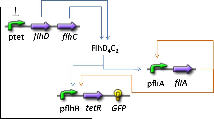
• We wanted to see if, from a mathematical point of view, it was possible for the "short" system presented above to hover.

• Here are the equations we took into account :

• The equations are normalized (thus the degradation term set to 1), as well as the parameters :

• At first, we quickly run simulations with different values of the parameters of the Hill function. Here are plot examples :
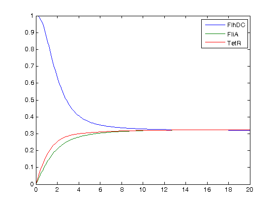
  • With n=2, we see no oscillations
    
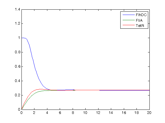
  • Here, with n=5, we begin to see some oscillations at the begining...

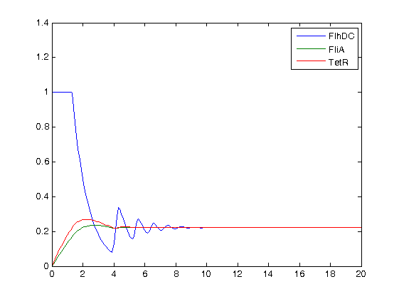
• • We then tried to increase drastically the value of n, to 300. Even though this had no biological reality, this met our simulating purpose

FIFO

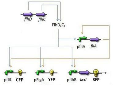
• The goal here is to present the results of the simulations we made concerning the FIFO part of the system.

Here is the system we implementated using Matlab (see the corresponding codes)

and the corresponding equations (for more detailed information see our establishment of the model).

where CFP, YFP, and RFP will be denoted below as respectively Z1,Z2 and Z3.

• We wanted to see if our predictions were accurate or not. We then solved the equations, forcing the behavior of FhlDC. In a first step, we imposed a constant production term of 1. Then, at a certain time, we set this production term to zero :

In fact we assumed that this behavior for FlhDC was acceptable regarding its estimated behavior in the whole system.

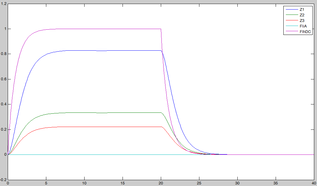
• We saw previously that without FliA, the FIFO would presumably not work. We then simulated a first system, where [FliA] stays to zero value.
  

We may see that there is a LIFO behavior rather than the FIFO we expect...

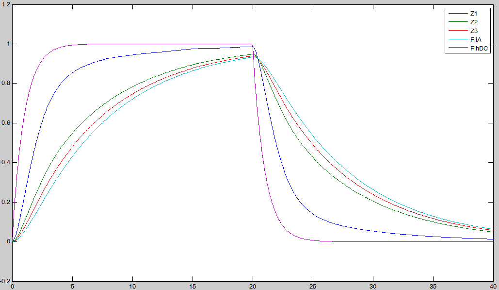
• Then, we simulated the entire system, to check if we had
  • the lasting burst due to FliA (more important for Z3 than for Z2, and more important for Z2 than Z1) in the increasing phase.
  • the effect of fliA which maintained the concentrations to their maximum (more important for Z3 than for Z2, and more important for Z2 than Z1) in the decreasing phase.
    

• We observe on these plots that the behavior is quite the one we expected, and that the FIFO is realized. FliA enables the curves to cross, and adds a delay on the genes that are most affected, with gives a better observability of the FIFO behavior.

Synchronisation

simul plsrs cells
Etude maths