Team:KULeuven/Model/Sensitivity
From 2008.igem.org
m |
|||
| Line 5: | Line 5: | ||
=== Episode I: The MATLAB Menace === | === Episode I: The MATLAB Menace === | ||
| - | Sensitivity analysis for Dr. Coli has been a pain in the ***. Our first attempts at this were done with the Sensitivity Analysis Tool that is included in MATLAB Simbiology. The problem here is that our model calls MATLAB's power fuction. Sensitivity analysis currently uses complex-step differentiation, which is currently not supported | + | Sensitivity analysis for Dr. Coli has been a pain in the ***. Our first attempts at this were done with the Sensitivity Analysis Tool that is included in MATLAB Simbiology. The problem here is that our model calls MATLAB's power fuction. Sensitivity analysis currently uses complex-step differentiation, which is currently not supported by this function. The computed sensitivities may not even approximate true sensitivities. So the value of this analyisis is doubtful. |
Nevertheless, below are some results of the calculated sensitivities for species in the system that precede any reaction that calls the power function. | Nevertheless, below are some results of the calculated sensitivities for species in the system that precede any reaction that calls the power function. | ||
| Line 33: | Line 33: | ||
A third situation has also been analysed. In the above two cases we constantly give 0 or 1 respectively. Our system however has a third and very important state: 0 - 1 - 0. In this state, the memory is ON and the timer can function. To simulate this, we used the same formula but we also created an event during the simulation. | A third situation has also been analysed. In the above two cases we constantly give 0 or 1 respectively. Our system however has a third and very important state: 0 - 1 - 0. In this state, the memory is ON and the timer can function. To simulate this, we used the same formula but we also created an event during the simulation. | ||
| - | These attempts | + | These attempts gave us more helpful results. We can even interpret something stability-like for our memory now: how far can our parameterisation be off before the memory stops functioning as expected. The results obtained by using this method for sensitivity analysis can be seen depicted in the figures below. |
==== Output ==== | ==== Output ==== | ||
Revision as of 12:12, 1 October 2008
Contents |
Sensitivity Analysis
Episode I: The MATLAB Menace
Sensitivity analysis for Dr. Coli has been a pain in the ***. Our first attempts at this were done with the Sensitivity Analysis Tool that is included in MATLAB Simbiology. The problem here is that our model calls MATLAB's power fuction. Sensitivity analysis currently uses complex-step differentiation, which is currently not supported by this function. The computed sensitivities may not even approximate true sensitivities. So the value of this analyisis is doubtful. Nevertheless, below are some results of the calculated sensitivities for species in the system that precede any reaction that calls the power function.
In these graphs, the 'parameters'-axis shows the parameters that are varied in the sensitivity analysis, while the ones along the states axis are the ones monitored as output. The z-axis is a measure for the sensitivity of the parameter under study.


Episode IV: A New Hope
We had come to the conclusion that the MATLAB sensitivity analysis just would not cut it for us, so we went on and started digging again. We tried a whole lot of different approaches, but nothing seemed to be appropriate for our system. (These attempts are episode II and III which we'll just skip here and forget about) Finally, we came up with the following. We define sensitivity in two different states, the ON state of the system and the OFF state The ON state receives maximal input during the entire simulation, while the OFF state only gets background signal. We come to the following formulae where X is the output species that we look at and P is the parameter that is changed to 110% or 90% of its own value. The second term is for normalisation purposes.
A third situation has also been analysed. In the above two cases we constantly give 0 or 1 respectively. Our system however has a third and very important state: 0 - 1 - 0. In this state, the memory is ON and the timer can function. To simulate this, we used the same formula but we also created an event during the simulation.
These attempts gave us more helpful results. We can even interpret something stability-like for our memory now: how far can our parameterisation be off before the memory stops functioning as expected. The results obtained by using this method for sensitivity analysis can be seen depicted in the figures below.
Output
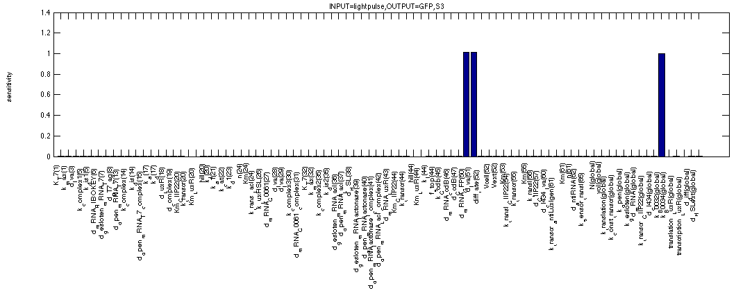
More as a control, the first figure depicts the sensitivity of our output GFP. It behaves completely as expected, clearly showing only dependencies for the degradation and synthesis rates of GFP while everything else is equal to zero. Also according to plan, the simulation gives exactly the same results for the two formulae above.
Memory
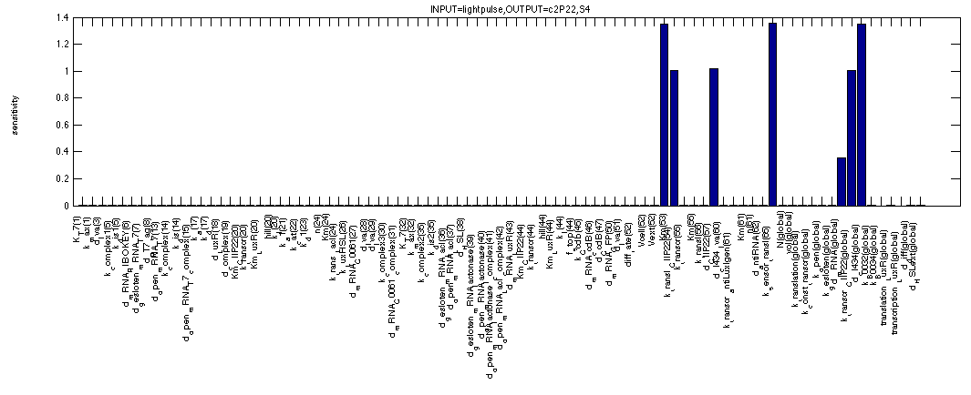
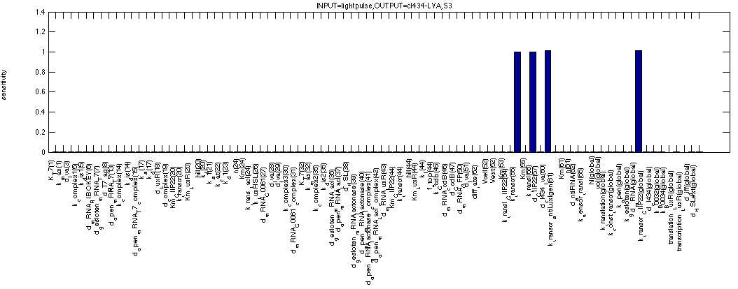
As mentioned before, we can use the sensitivity analysis of the memory to see how big our margins are on the arious parameters that make out our model. The first figure shows the sensitivity of c2 P22 for all system parameters in the OFF state. This means we use the second formula. The analysis shows all expected dependencies such as synthesis and degradation rates for c2 P22. But also for the affinity of cI 434 for the promoter in front of c2 P22, for the production/degradation rates of cI 434 with(out) LVA tag.
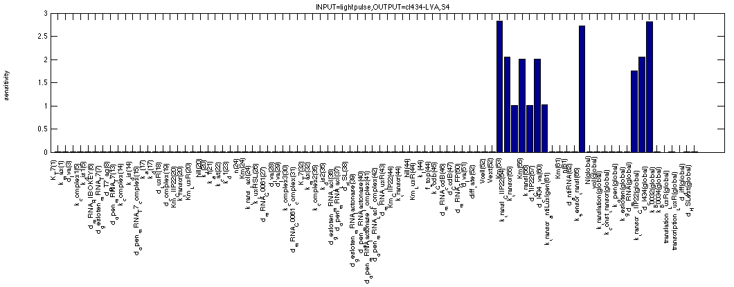
For cI 434 in the OFF state, we see similar but distinct results. We see that all sensitivities appear to be bit higher and that some extra factors have appeared describing repression by and degradation of c2 P22 repressor. Once again logical results.
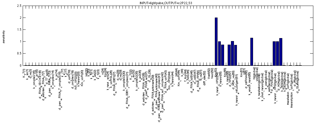
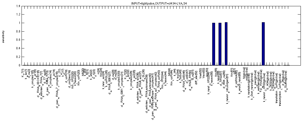
The next figure shows the sensitivities for c2 P22 in the ON state of the memory (where it plays a similar role as cI 434 (LVA) in the OFF state). We can even see that the figure is very similar to the one just above, except that the affinity of c2 P22 for the promoter controlling cI 434 (LVA) doesn't seem to matter anymore. This can be easily understood if you remember that we're simulating a continuous 1 signal here, where a lot of cI 434 (without LVA) is coming from the TetR promoter, making small contributions to the cI 434 concentration by the c2 P22 repressible promoter quite irrelevant in this case.
cI 434 (without LVA tag) during a continuous 1 signal is only dependent on the obvious synthesis, degradation rates as can be expected with the total amount of cI 434 being high enough to remove all c2 P22 from the system.
A final figure shows the sensitivity of the same cI 434 without tag in a system that has been activated but is now without input. The switch appears to be so strong that we only detect the same sensitivities as in the above scenario of a continuous 1 signal.
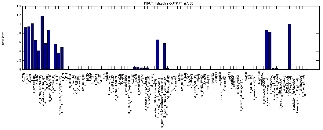
The first figure shows the sensitivities for Lactonase in the ON state (the first formula). They can all be expected; we clearly see the dependence on the filter (T7 as well as key-lock characteristics) as well as more obvious synthesis and degradation rates of lactonase itself.
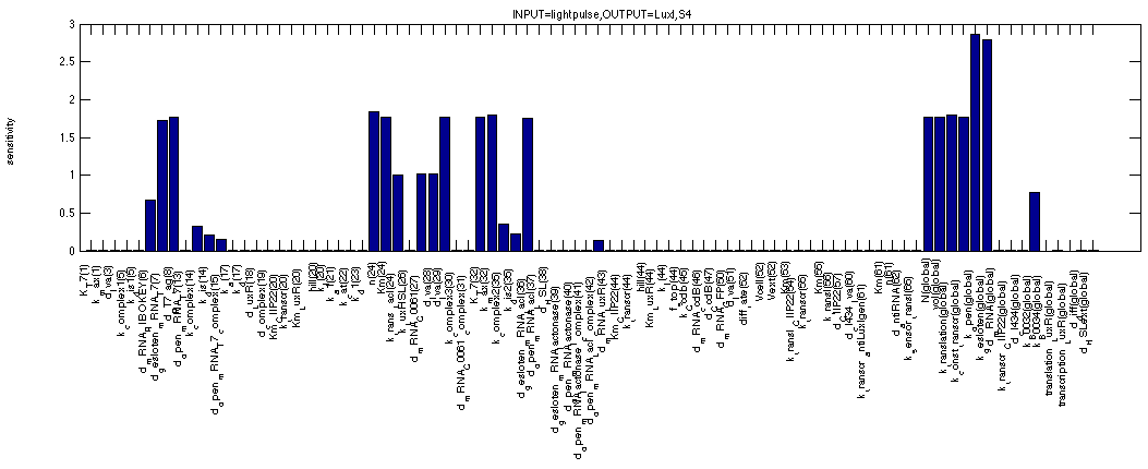
This next one shows the sensitivities of LuxI in a 0 - 1 - 0 event situation. We clearly see the filter effect again but this time it appears to be reinforced by the LacI repressor of the inverter. The parameters for LacI repression are also nicely visible.
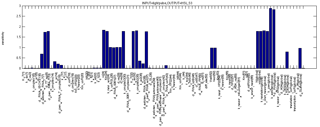
By looking at HSL in the same 0 - 1 - 0 scenario, we see a very similar picture. All the same sensitivities are visible plus three significant new ones. The first is obvious, it is the rate of HSL synthesis by LuxI. The other two are less obvious, they are the cell volume and the volume of the medium. These are effects of the diffusion out of the cell and into the medium.
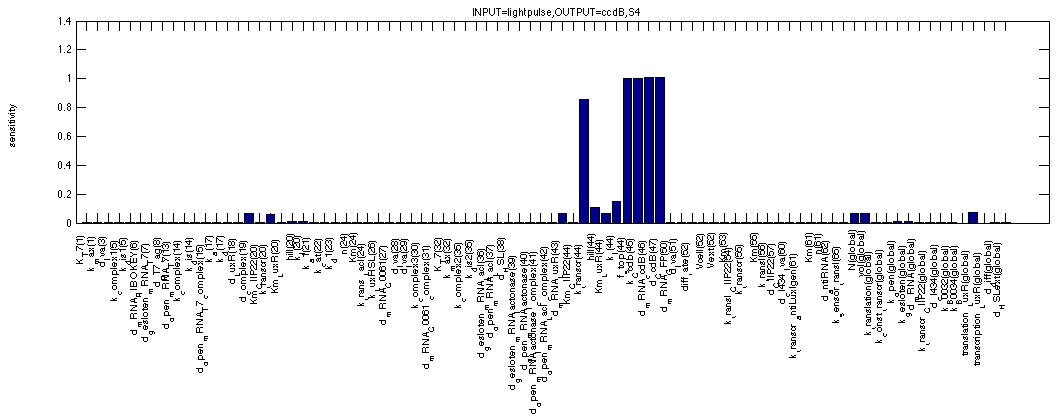
The final study is of ccdB, our final effector in the 0 - 1 - 0 scenario. We can see small sensitivities for the parameters characterising the HSL-LuxR complex such as affinity of the complex for the DNA, affinity of HSL for LuxR etc. The highest sensitivities we get for the properties of ccdB itself. The terminator efficiency and other synthesis and degradation rates.
Further conclusions
Our model seems to respond to these sensitivity analyses as suspected and at first glance appears to give us a bit of a margin on most of our parameters.
 "
"


