Team:KULeuven/Model/Overview
From 2008.igem.org
m |
m |
||
| Line 4: | Line 4: | ||
__NOTOC__ | __NOTOC__ | ||
| - | |||
| - | |||
=== Introduction === | === Introduction === | ||
Revision as of 14:59, 3 October 2008
Introduction
As an introduction to modeling we've made a small presentation for the workout sessions of the first meeting. This presentation handles the following items:
- some definitions
- the difference between white box and black box models with an example
- focus on the role of ODE's
- the need for modeling
- some modeling tools
- and iGEM modeling
This presentation is mainly based on the wiki of ETH Zürich 2006/2007.
The Full Model
Modeling steps
Position in the system
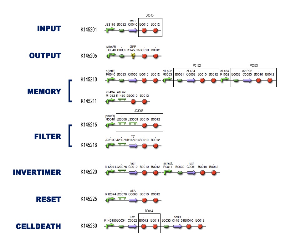
For each of the subsystems (compartments) we started with the idea of what it was supposed to do, considering it as a black-box system (as described in the project page). To make sure that Dr. Coli was able to do his work properly, we had to design several subsystems and be well aware of the different interfaces between these subsystems.
Then we tried to match species with these black-boxes, keeping in mind the working biobricks which have been made already. So we searched for existing components which could be able to perform the requested task.
Describing the system
The kinetic actions (transcription, translation, complexation, ...) that take place in the subsystems can be described by Ordinary Differential Equations (ODEs) like Mass-Action laws, Hill Kinetic laws and so on. An extensive search for parameters involved in these ODEs has resulted in the discovery of almost all necessary quantities for the simulations.
For every subsystem, we made a PDF-file with all the ODEs involved in modeling the subsystem, together with a clear overview of the used parameters (with coherent links to our references).
Models
We implemented these ODEs in both [http://www.systems-biology.org/cd/ Celldesigner] and the [http://www.mathworks.com/access/helpdesk/help/toolbox/simbio/ MATLAB Symbiology Toolbox]. A nice tutorial for modeling in Celldesigner can be found on [http://openwetware.org/wiki/Imperial_College/Courses/Spring2008/Synthetic_Biology/Computer_Modelling_Practicals Imperial College Computer Modelling Practicals Spring 2008]. These 2 environments offer a grapical user-interface which makes it easy to implement biochemical pathways (and the kinetic laws which govern these). In the pictures in each of the subsytems you can see clearly the influence of the different species: activation, repression, complexation, ... We also provide links to the actual implemented diagrams which can be freely downloaded to simulate the subsystems yourself.
Simulation(s)
The implemented models are simulated using inputs as close to reality as possible. In each simulation the typical assets of each subsystem are clearly visualized and described extensively. For example in the filter we simulate the influence of different noisy signals on the output of the filter (and on the output of the system).
Sensitivity Analysis
Good modeling practice requires that the modeler provides an evaluation of the confidence in the model, possibly assessing the uncertainties associated with the modeling process and with the outcome of the model itself. Uncertainty and Sensitivity Analysis offer valid tools for characterizing the uncertainty associated with a model. Uncertainty analysis (UA) quantifies the uncertainty in the outcome of a model. Sensitivity Analysis has the complementary role of ordering by importance the strength and relevance of the inputs in determining the variation in the output. Sensitivity analysis lets you calculate the time-dependent sensitivities of all the species states with respect to species initial conditions and parameter values in the model.
A sensitivity analysis is needed e.g. when some of the parameter values are not known. The true value of a parameter is unimportant when the most essential species states are insensitive to the unknown parameter. Only for the sensitive unknown parameters are experiments needed to determine their true values. In our project we have been able to find hypothetical values for all used parameters, but a sensitivity analyses is nevertheless always valuable to detect critical parameters. These are the parameter values on which our project critically depends and which should be analyzed/characterized as exact as possible.
Our analysis is based upon the following formulae where X is the output species that we look at and P is the parameter that is changed to 110% or 90% of its own value. The second term is for normalisation purposes. Results and discussions can be found in the appropriate section.
Important notes
1. The idea of a pulsgenerator as reset mechanism has been cancelled for the following reasons:
- it takes too long before the proposed system generates a pulse-like event
- the pulse itself is too long
- a constant lactonase production sequence generates enough lactonase to reset the timer
More information about this problem and the solution can be found on Reset-page.
2. A mathematical analyses of the memory has been done to prove that it has 2 stable states and to describe the boundary which separates the trajectories leading to one of the steady states.
More information about this analysis can be found on Memory-page.
 "
"


