Team:Paris/Modeling/BOB/Simulations page travail
From 2008.igem.org
(→Observations) |
|||
| Line 47: | Line 47: | ||
=== Observations === | === Observations === | ||
| - | * First of all, let us see what the simulation gives, and what pieces of information we can get from it. | + | * Observation#1: |
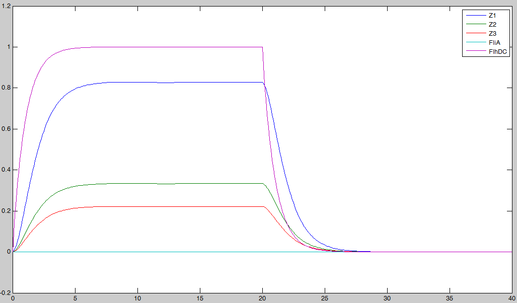
| + | First of all, let us see what the simulation gives, and what pieces of information we can get from it. | ||
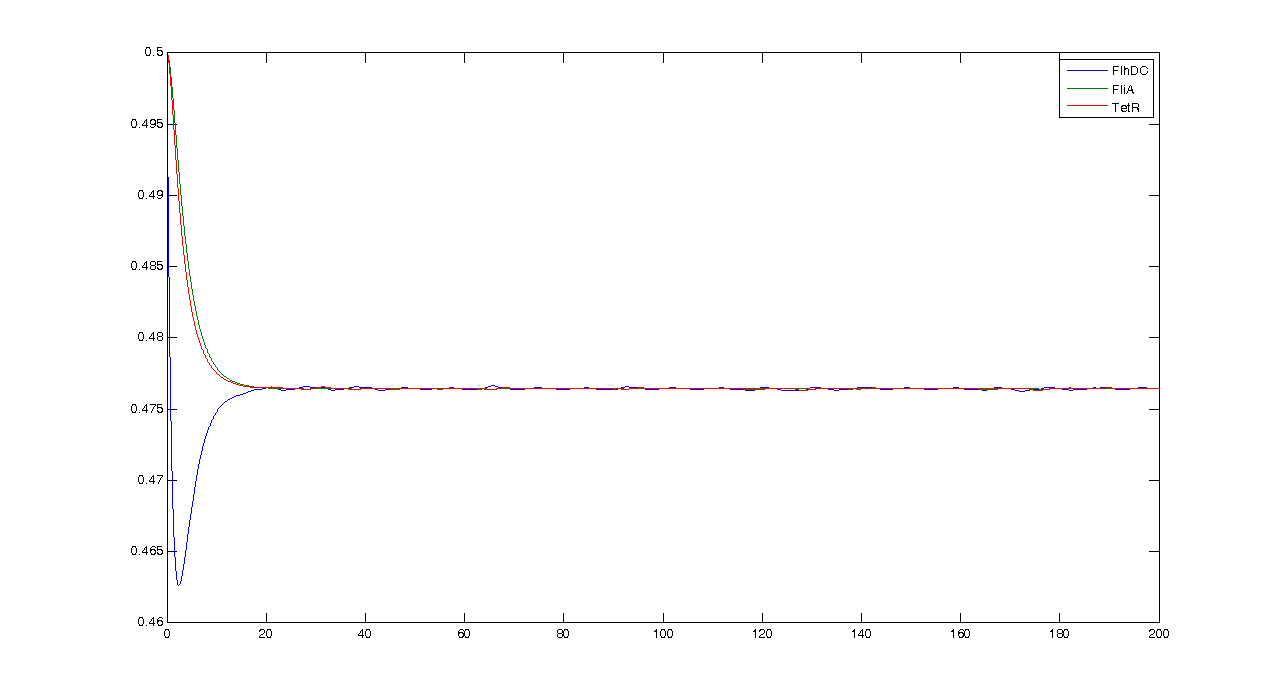
By looking at this simulation, we could think that it is going to be hard to get oscillations...[[Image:Simul_fig1_re.jpg|900px|center]] | By looking at this simulation, we could think that it is going to be hard to get oscillations...[[Image:Simul_fig1_re.jpg|900px|center]] | ||
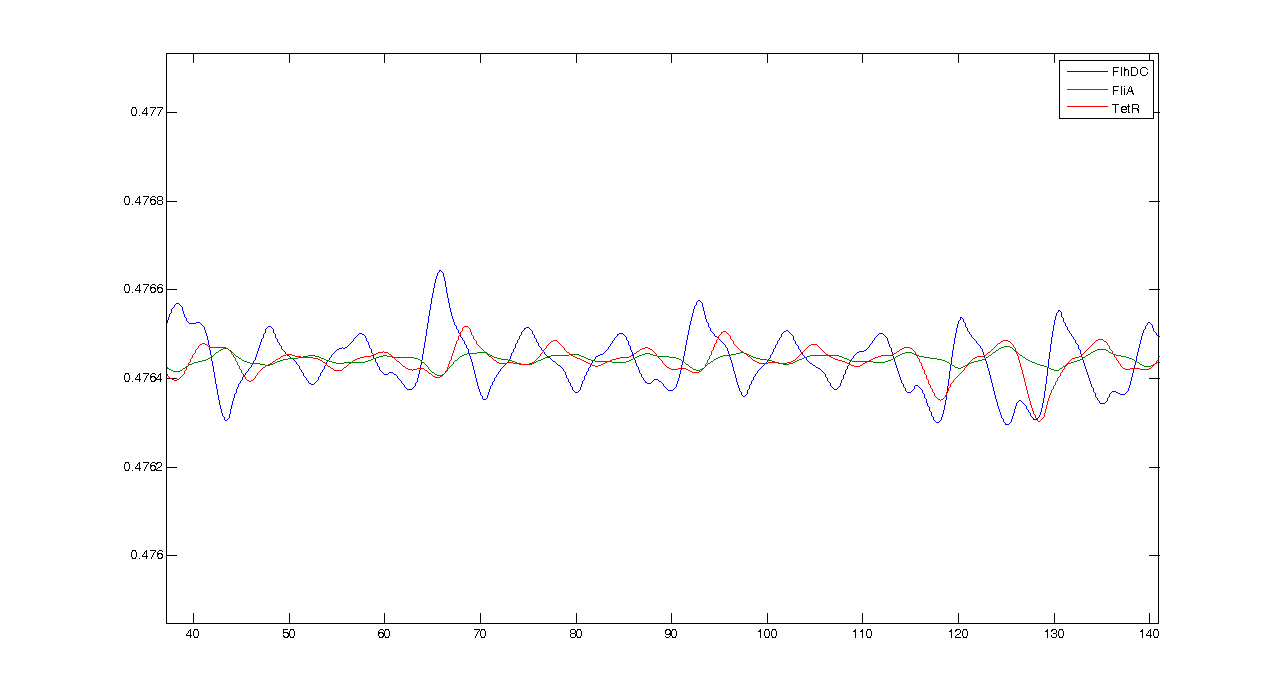
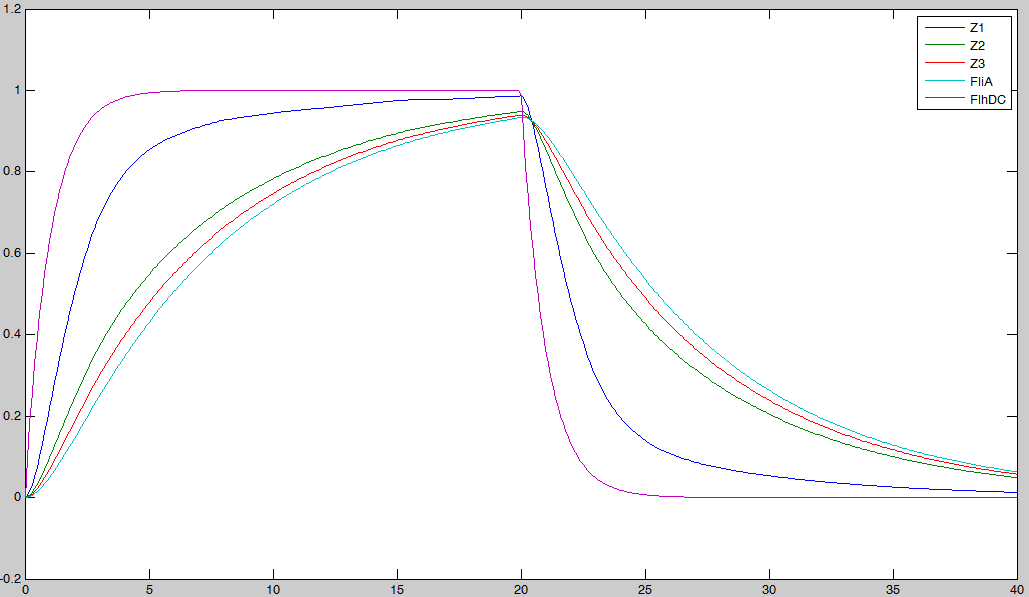
However when we zoom, we get this more reassuring view :[[Image:Simul_fig2_re.jpg|900px|center]] | However when we zoom, we get this more reassuring view :[[Image:Simul_fig2_re.jpg|900px|center]] | ||
| - | + | Conclusion : some intrinsic oscillations actually occur, but they seem to be strongly attenuated. The mathematical study shall help us decide whether these are only artefact oscillations. For example we shall try to check if the period observed (~10 time units) can be linked to mathematical data. | |
| + | * Observation#2 | ||
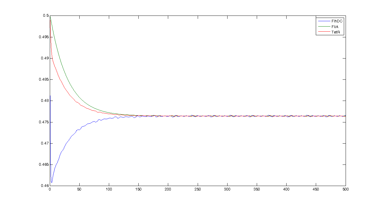
| + | There is another relevant question: which of the three promoters we have (pFliL, pFlgA, pFlhB) is the best. Here is a comparison of the simulation for the three systems: | ||
| + | [[Image:simul_compar_fliL.jpg|600px|center|thumb|pFliL]] | ||
| + | [[Image:simul_compar_flgA.jpg|600px|center|thumb|pFlgA]] | ||
| + | [[Image:simul_compar_flhB.jpg|600px|center|thumb|pFlhB]] | ||
=== Understanding the dynamics === | === Understanding the dynamics === | ||
Revision as of 01:57, 9 October 2008
|
Simulations and Mathematical analysis
OscillationsShort System
Observations
First of all, let us see what the simulation gives, and what pieces of information we can get from it. By looking at this simulation, we could think that it is going to be hard to get oscillations... However when we zoom, we get this more reassuring view :Conclusion : some intrinsic oscillations actually occur, but they seem to be strongly attenuated. The mathematical study shall help us decide whether these are only artefact oscillations. For example we shall try to check if the period observed (~10 time units) can be linked to mathematical data.
There is another relevant question: which of the three promoters we have (pFliL, pFlgA, pFlhB) is the best. Here is a comparison of the simulation for the three systems: Understanding the dynamics
The classical approach consists in finding the equilibrium state, by setting Then, we evaluate the jacobian matrix, so as to put the system under its linearized form:
which gives : Then, we want to find the eigenvalues of the jacobian matrix, because they make us understand the behavior of the system. Here is the theoretical explanation : The λ and γ coefficients make the convergence. In our case they are negative terms, which explains the fact that we have a quick convergence for the system. Ideally, it could be convenient to find which parameter influence this coefficient, so as to play with it and be able to propose a better control of the convergence.
We obtained three solutions : -0.2382 - 0.6139i -0.2382 + 0.6139i 0.4764 We are only interested in positive real solutions. We can note that 0.4764 corresponds well to the experimental equilibrium value. Then we evaluated the eigenvalues for the jacobian : -1.0159 + 0.5042i -1.0159 - 0.5042i -0.1111 We can note that the λ and γ coefficient are negative, which corroborates the fact that we obtain a convergence. Finally for since μ=0.5042 we find a theoretical period of Ttheoretical=12.4617. Experimentally, we find Texperimental~10. We can see that some numerical noise must be involved, which gives the reading of the period quite tough. However, we get the same order of magnitude, which proves that the oscillations are occuring, though quietly!
Furthermore, this theoretical study helps us understand that reducing the attenuation is tough. In fact, whatever the base in which you consider a matrix, the trace is conserved. Here, we obtain : Since λ and γ are assumed (thanks to simulations) to be negative, we cannot avoid to have their sum to be (with absolute value) superior to 2. The only chance we have would be that the weight goes in the λ parameter because this parameter plays a role in the third dimension, in which we are not interested. However, for every simulation we made, we found the opposite. Trying to evaluate with non-numerical calculus does not provide relevant material. However, we now know that βFliA influences the attenuation. We ran a simulation with βFliA=0.02 This confirms what we saw previously. Before, the system was hovering around the equilibrium at T=20. In this second case, the system is therefore less attenuated, and we have to wait until T=150 to observe the effect. Last but not least, one should not forget that we chose a normalized interpretation of the system. Thus, even though the attenuation phenomenon remains unchanged, the tiny oscillations we see may indeed be observable. Using these elements to improve the system and give directions to the wet-lab
VOIR SI ON PEUT FAIRE l'algo Entire System//biocham ici//+ comparaison avec le modele hillistique FIFO
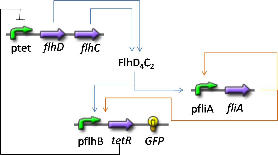
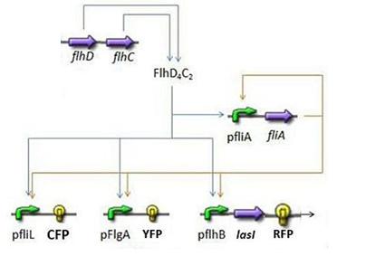
Here is the system we implementated using Matlab (see the corresponding codes) and the corresponding equations (for more detailed information see our establishment of the model). where CFP, YFP, and RFP will be denoted below as respectively Z1,Z2 and Z3.
In fact we assumed that this behavior for FlhDC was acceptable regarding its estimated behavior in the whole system.
We may see that there is a LIFO behavior rather than the FIFO we expect...
SynchronizationMathematical AnalysisSimulations and verification of the hypothesis |
|||||||||||||||||||
 "
"

