|
Simulations and Mathematical analysis
Oscillations
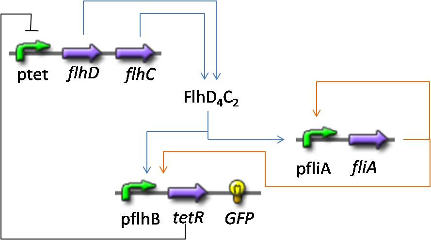
Short System
- We wanted to see if, from a mathematical point of view, it was possible for the "short" system presented above to hover.
- Here are the equations we took into account :
- The equations are normalized (thus the degradation term set to 1), as well as the parameters :
| Parameters Used
|
| Parameter
| Normalized Value
|
| βFlhDC
| 1
|
| θFlhDC
| 0.4545
|
| n
| 2
|
| βFliA
| 0.1429
|
| β'FliA
| 0.8581
|
| βLasI
| 0.2222
|
| β'LasI
| 0.7778
|
- As introduced before, the goal of this model was to give us useful bases on which to work on. Then, we shall use the values of the parameters presented below as a "starting point". We shall present a double approach, composed of a theoretical and a simulation approach. Both approaches should interact so as to help us understand the way our system behaves.
- The obvious though process we propose consists in observing what happens with the simulation, then understand the source of these phenomenas. Finally, the ultimate goal consists in finding how we can pull the strings, hidden in the system, that control the behavior of the system.
Observations
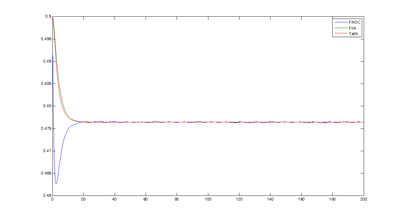
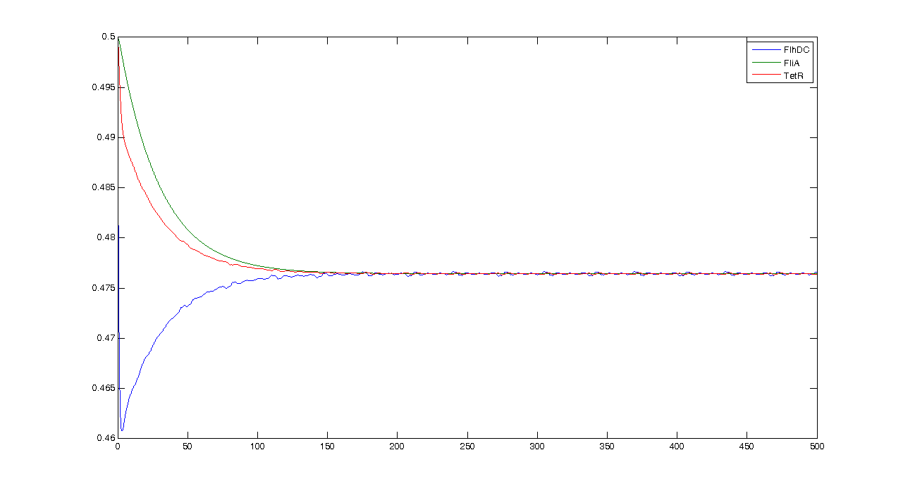
First of all, let us see what the simulation gives, and what pieces of information we can get from it.
By looking at this simulation, we could think that it is going to be hard to get oscillations...
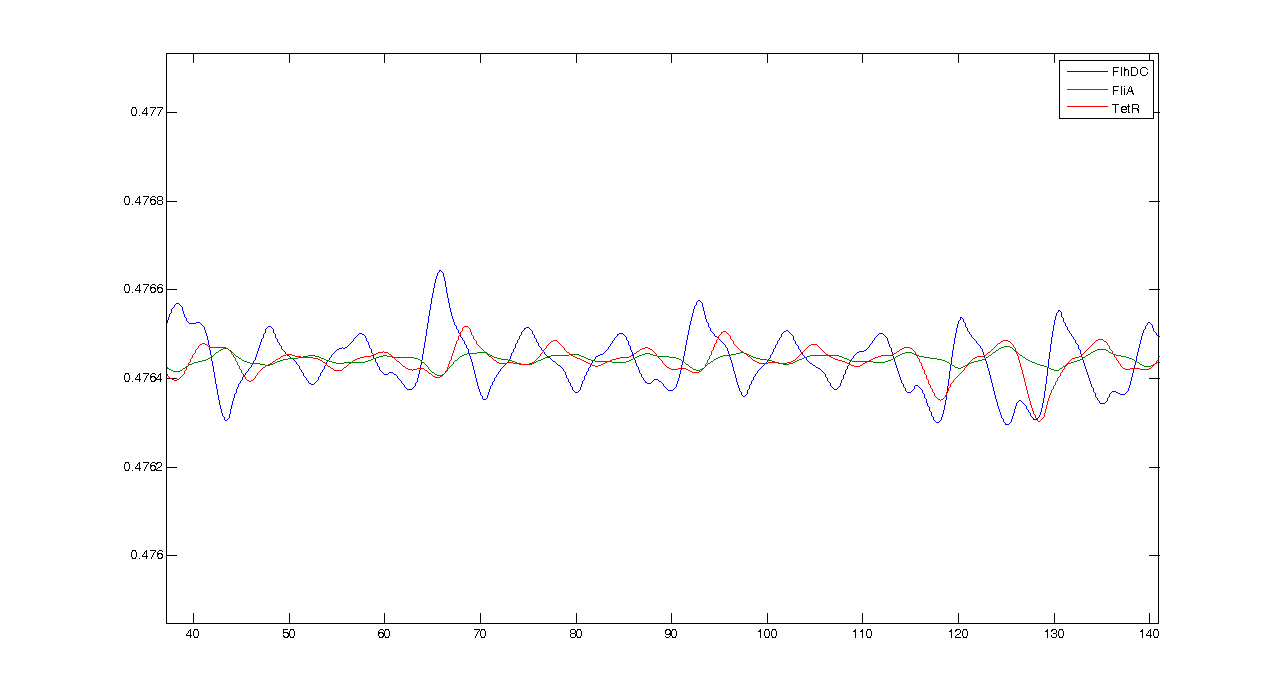
However when we zoom, we get this more reassuring view :
Conclusion : some intrinsic oscillations actually occur, but they seem to be strongly attenuated. The mathematical study shall help us decide whether these are only artefact oscillations. For example we shall try to check if the period observed (~10 time units) can be linked to mathematical data.
There is another relevant question: which of the three promoters we have (pFliL, pFlgA, pFlhB) is the best. Here is a comparison of the simulation for the three systems:
| pFliL
|
| equilibrium state
| 0.4764
|
| λ
| -0.0722
|
| γ + iμ
| -1.0353 + 0.9523i
|
| γ + iμ
| -1.0353 - 0.9523i
|
| pFlgA
|
| equilibrium state
| 0.4764
|
| λ
| -0.1007
|
| γ + iμ
| -1.0211 + 0.6139i
|
| γ - iμ
| -1.0211 - 0.6139i
|
| pFlhB
|
| equilibrium state
| 0.4764
|
| λ
| -0.1111
|
| γ + iμ
| -1.0159 + 0.5042i
|
| γ - iμ
| -1.0159 - 0.5042i
|
To conclude, we obtained highly interesting data. Going from pFliL to pFlhB, the further we go, the more chaotic the oscillations are. With pFliL, the oscillations are neat, regular. With pFlHB, they are more noised. Consequently, here is a new data that can be given to the wet-lab so as to build the best system.
Understanding the dynamics
The classical approach consists in finding the equilibrium state, by setting
Then, we evaluate the jacobian matrix, so as to put the system under its linearized form:
which gives :
Then, we want to find the eigenvalues of the jacobian matrix, because they make us understand the behavior of the system. Here is the theoretical explanation :
The λ and γ coefficients make the convergence. In our case they are negative terms, which explains the fact that we have a quick convergence for the system. Ideally, it could be convenient to find which parameter influence this coefficient, so as to play with it and be able to propose a better control of the convergence.
The μ coefficient is responsible for the oscillations. In fact, in another base, with only real matrix, this would beget cosinuses and sinuses terms. Furthermore, it is strongly linked to the period of the oscillations.
- Comparison of the simulation and theoretical periods
We can hereby prove that the small oscillations observed before are not induced by a simulation artefact, by evaluating the theoretical value of the period. Indeed, we have: With the parameters presented in the array before, we have evaluated the equilibrium values by solving
We obtained three solutions :
-0.2382 - 0.6139i
-0.2382 + 0.6139i
0.4764
We are only interested in positive real solutions. We can note that 0.4764 corresponds well to the experimental equilibrium value.
Then we evaluated the eigenvalues for the jacobian :
-1.0159 + 0.5042i
-1.0159 - 0.5042i
-0.1111
We can note that the λ and γ coefficient are negative, which corroborates the fact that we obtain a convergence.
Finally for since μ=0.5042 we find a theoretical period of Ttheoretical=12.4617. Experimentally, we find Texperimental~10. We can see that some numerical noise must be involved, which gives the reading of the period quite tough. However, we get the same order of magnitude, which proves that the oscillations are occuring, though quietly!
- Understanding the attenuation
Furthermore, this theoretical study helps us understand that reducing the attenuation is tough. In fact, whatever the base in which you consider a matrix, the trace is conserved. Here, we obtain :
Since λ and γ are assumed (thanks to simulations) to be negative, we cannot avoid to have their sum to be (with absolute value) superior to 2. The only chance we have would be that the weight goes in the λ parameter because this parameter plays a role in the third dimension, in which we are not interested. However, for every simulation we made, we found the opposite. Trying to evaluate with non-numerical calculus does not provide relevant material.
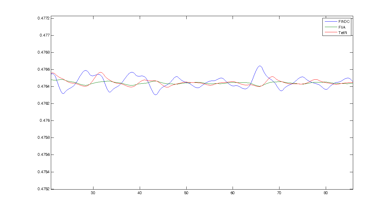
However, we now know that βFliA influences the attenuation. We ran a simulation with βFliA=0.02
This confirms what we saw previously. Before, the system was hovering around the equilibrium at T=20. In this second case, the system is therefore less attenuated, and we have to wait until T=150 to observe the effect.
Last but not least, one should not forget that we chose a normalized interpretation of the system. Thus, even though the attenuation phenomenon remains unchanged, the tiny oscillations we see may indeed be observable.
Using these elements to improve the system and give directions to the wet-lab
- First and foremost, we learnt that the best promoter to use is pFliL. As far as the biological construction is concerned, we argue that this promoter would give the best chances of success.
- Then, To what extent can this study help us improve our oscillations? We want to minimize the γ coefficient, and we know that the period is linked to the μ coefficient.
- Therefore, we understood that βFliA had a considerable influence over the attenuation. Therefore, this enables us to ask the wet-lab to try minimize this parameter. In addition, we set the degradation terms to 1. Even though they do not appear in the equations presented before, they have the same influence as βFliA since in reality we have λ + 2γ = - (∑(degradation terms) + βFliA).
- Then, the ideal though process would be to get the equilibrium state, but not with numerical values, so as to understand the influence of each of the system parameter. However, we face a major problem since this would require to solve an (n+1) degree equation, which explicit solutions are useless. Yet, imagining that we can get the solution, we could evaluate the eigenvalues in the same way (since they are solution of a third degree equation, this could be possible). Consequently, we could understand the influence of each parameter, and we could find a way to minimize the our γ coefficient.
As a matter of facts, we understand that even though we consider the short system, this process faces strong difficulties. Yet, it is possible to consider an algorithmic approach that meets the same ends.
- We have the parameters which we want to change to evolve gradually between extreme values (that are definitely not biologically coherent)
- we run the estimation of the equilibrium state, and we get the eigenvalues
- we keep the parameters that beget the smallest value for γ
Finally we see with the wet-lab how we can play biologically to change thoses parameters in the way we designed.
VOIR SI ON PEUT FAIRE l'algo
Entire System
//biocham ici//+ comparaison avec le modele hillistique
FIFO
- The goal here is to present the results of the simulations we made concerning the FIFO part of the system.
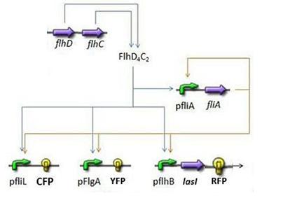
Here is the system we implementated using Matlab (see the corresponding codes)
and the corresponding equations (for more detailed information see our establishment of the model).
where CFP, YFP, and RFP will be denoted below as respectively Z1,Z2 and Z3.
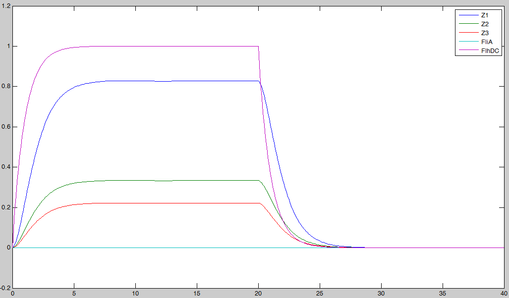
- We wanted to see if our predictions were accurate or not. We then solved the equations, forcing the behavior of FhlDC. In a first step, we imposed a constant production term of 1. Then, at a certain time, we set this production term to zero :
In fact we assumed that this behavior for FlhDC was acceptable regarding its estimated behavior in the whole system.
- We saw previously that without FliA, the FIFO would presumably not work. We then simulated a first system, where [FliA] stays to zero value.
We may see that there is a LIFO behavior rather than the FIFO we expect...
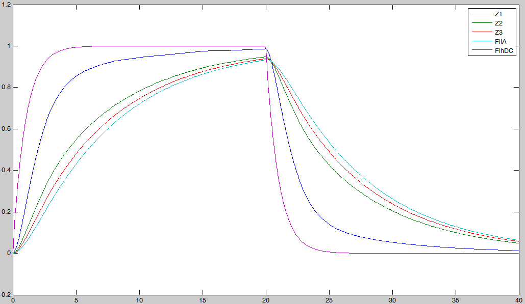
- Then, we simulated the entire system, to check if we had
- the lasting burst due to FliA (more important for Z3 than for Z2, and more important for Z2 than Z1) in the increasing phase.
- the effect of fliA which maintained the concentrations to their maximum (more important for Z3 than for Z2, and more important for Z2 than Z1) in the decreasing phase.
- We observe on these plots that the behavior is quite the one we expected, and that the FIFO is realized. FliA enables the curves to cross, and adds a delay on the genes that are most affected, with gives a better observability of the FIFO behavior.
Synchronization
Mathematical Analysis
Simulations and verification of the hypothesis
|
 "
"

