|
|
| (18 intermediate revisions not shown) |
| Line 1: |
Line 1: |
| - | [[Image:f3env.png|thumb]] (see [[Team:Paris/Modeling/Oscillations#Biochemical_Assumptions|the considerations on the use of EnvZ]])
| + | {{Paris/Menu}} |
| | | | |
| - | We have [EnvZ]<sub>produced</sub> = {coef<sub>env</sub>}''expr(pTet)'' = {coef<sub>env</sub>} ƒ1([aTc]<sub>i</sub>)
| + | {{Paris/Header|Method & Algorithm : ƒ3bis}} |
| | + | <center> = act_''pFlhDC'' </center> |
| | + | <br> |
| | | | |
| - | and [EnvZ]<sub>total</sub> = [EnvZ]<sub>basal</sub> + [EnvZ]<sub>produced</sub>
| + | [[Image:f6DCA.png|thumb|Specific Plasmid Characterisation for ƒ3bis]] |
| | + | In this experiment, we have |
| | | | |
| - | and [FliA] = {coef<sub>FliA</sub>}''expr(pBad)'' = {coef<sub>FliA</sub>} ƒ2([arab]<sub>i</sub>)
| + | ''' [''EnvZ'']<sub>''real''</sub> = {coef<sub>''envZ''</sub>} ƒ1([aTc]<sub>i</sub>) ''' |
| | | | |
| - | So, if we denote phosphorylated OmpR by ''OmpR<sup>*</sup>'', we have
| + | but we use ''' [aTc]<sub>i</sub> = Inv_ƒ1( [''EnvZ''] ) ''' |
| | | | |
| - | [[Image:F3ompfromenv.jpg|center]]
| + | so, at steady-states, ''phosphorylated OmpR'' verify : |
| | | | |
| - | that we can then introduce in the previous expression (ƒ 3) :
| + | [[Image:F3b.jpg|center]] |
| | | | |
| - | [[Image:F3ompfinal.jpg|center]] | + | We can then solve it, and reintroduce the result in the previously characterized ''' ƒ3( 0, [OmpR<sup>*</sup>] ) ''', to determine the parameters : |
| | | | |
| - | <br><br> | + | <div style="text-align: center"> |
| | + | {{Paris/Toggle|Table of Values|Team:Paris/Modeling/More_f3bis_Table}} |
| | + | </div> |
| | | | |
| - | {|border="1" style="text-align: center"
| + | <div style="text-align: center"> |
| - | |param
| + | {{Paris/Toggle|Algorithm|Team:Paris/Modeling/More_f3bis_Algo}} |
| - | |signification
| + | </div> |
| - | |unit
| + | |
| - | |value
| + | |
| - | |-
| + | |
| - | |[expr(pFlhDC)]
| + | |
| - | |expression rate of <br> pFlhDC '''with RBS E0032'''
| + | |
| - | |nM.s<sup>-1</sup> | + | |
| - | |see [[Team:Paris/Modeling/Programs|"findparam"]] <br> need for 20 + 20 measures <br> and 5x5 measures for the ''SUM''? | + | |
| - | |-
| + | |
| - | |γ<sub>GFP</sub>
| + | |
| - | |dilution-degradation rate <br> of GFP(mut3b)
| + | |
| - | |min<sup>-1</sup>
| + | |
| - | |0.0198
| + | |
| - | |-
| + | |
| - | |[GFP]
| + | |
| - | |GFP concentration at steady-state
| + | |
| - | |nM
| + | |
| - | |need for 20 + 20 measures <br> and 5x5 measures for the ''SUM''?
| + | |
| - | |-
| + | |
| - | |(''fluorescence'')
| + | |
| - | |value of the observed fluorescence
| + | |
| - | |au
| + | |
| - | |need for 20 + 20 measures <br> and 5x5 measures for the ''SUM''?
| + | |
| - | |-
| + | |
| - | |''conversion''
| + | |
| - | |conversion ratio between <br> fluorescence and concentration
| + | |
| - | |nM.au<sup>-1</sup>
| + | |
| - | |(1/79.429)
| + | |
| - | |}
| + | |
| | | | |
| - | <br><br>
| + | <br> |
| | | | |
| - | {|border="1" style="text-align: center"
| + | <center> |
| - | |param
| + | [[Team:Paris/Modeling/Implementation| <Back - to "Implementation" ]]| <br> |
| - | |signification <br> corresponding parameters in the [[Team:Paris/Modeling/Oscillations#Resulting_Equations|equations]]
| + | [[Team:Paris/Modeling/Protocol_Of_Characterization| <Back - to "Protocol Of Characterization" ]]| |
| - | |unit | + | </center> |
| - | |value
| + | |
| - | |-
| + | |
| - | |β<sub>12bis</sub>
| + | |
| - | |production rate of FliA-pFlhDC '''with RBS E0032''' <br> replace β<sub>12</sub> (not written)
| + | |
| - | |nM.min<sup>-1</sup>
| + | |
| - | |
| + | |
| - | |-
| + | |
| - | |(K<sub>11bis</sub>/{coef<sub>fliA</sub>})
| + | |
| - | |activation constant of FliA-pFlhDC <br> K<sub>11bis</sub> | + | |
| - | |nM
| + | |
| - | |
| + | |
| - | |-
| + | |
| - | |n<sub>11bis</sub> | + | |
| - | |complexation order of FliA-pFlhDC <br> replace n<sub>11</sub> (not written)
| + | |
| - | |no dimension
| + | |
| - | |
| + | |
| - | |-
| + | |
| - | |-
| + | |
| - | |β<sub>2bis</sub>
| + | |
| - | |production rate of EnvZ-pFlhDC '''with RBS E0032''' <br> β<sub>2bis</sub>
| + | |
| - | |nM.min<sup>-1</sup>
| + | |
| - | |
| + | |
| - | |-
| + | |
| - | |(K<sub>19bis</sub>/{coef<sub>envZ</sub>})
| + | |
| - | |activation constant of EnvZ-pFlhDC <br> replace K<sub>19</sub> (not written)
| + | |
| - | |nM
| + | |
| - | |
| + | |
| - | |-
| + | |
| - | |n<sub>19bis</sub>
| + | |
| - | |complexation order of EnvZ-pFlhDC <br> n<sub>19bis</sub>
| + | |
| - | |no dimension
| + | |
| - | |
| + | |
| - | |}
| + | |
| - | | + | |
| - | <br><br>
| + | |
| - | | + | |
| - | Then, if we have time, we want to verify the expected relation
| + | |
| - | | + | |
| - | [[Image:SumpFlhDC2.jpg|center]]
| + | |
|
Method & Algorithm : ƒ3bis
= act_pFlhDC
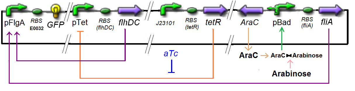 Specific Plasmid Characterisation for ƒ3bis In this experiment, we have
[EnvZ]real = {coefenvZ} ƒ1([aTc]i)
but we use [aTc]i = Inv_ƒ1( [EnvZ] )
so, at steady-states, phosphorylated OmpR verify :
We can then solve it, and reintroduce the result in the previously characterized ƒ3( 0, [OmpR*] ) , to determine the parameters :
↓ Algorithm ↑
function optimal_parameters = find_f3_EnvZ(X_data, Y_data, initial_parameters)
global beta17 K15 n15;
function output = act_pFlhDC(parameters, X_data)
for k = 1:length(X_data)
OmpR_P = complexes((parameters(1) + X_data(k)),parameters(2),parameters(3),parameters(4));
output(k) = beta17*(1 - hill( OmpR_P, K15, n15 ));
end
end
options=optimset('LevenbergMarquardt','on','TolX',1e-10,'MaxFunEvals',1e10,'TolFun',1e-10,'MaxIter',1e4);
optimal_parameters = lsqcurvefit( @(parameters, X_data) act_pFlhDC(parameters, X_data), ...
initial_parameters, X_data, Y_data, options );
end
|
<Back - to "Implementation" |
<Back - to "Protocol Of Characterization" |
|
 "
"

