Team:TUDelft/Color modeling
From 2008.igem.org
Contents |
Introduction
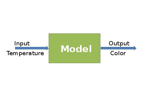
The model of biothermometer is included an input and output. The input of the model is the enzyme synthesis controlled by the temperature and the output is color production. The challenges for the modeling part are:
- Finding a suitable model for a temperature dependence synthesis for the color producing enzymes.
- Solving the Michaelis-Menten kinetic equations to obtain the dynamics of pathway intermediates.
The procedure for modeling was started with the output part, color pathway, and continued to the enzyme synthesis which can be controlled by temperature.
Color Modeling
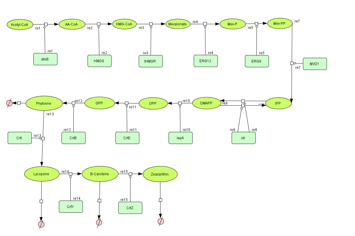
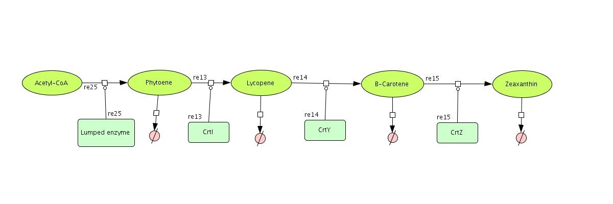
In the output we use [http://www.lbl.gov/Science-Articles/Archive/assets/images/2004/Mar-24/Engineering_terpenoids.pdf mevalonate] and [http://parts.mit.edu/igem07/index.php/Image:Zeaxanthin.jpg GPP] pathways together to produce red, orange and yellow colors. The biosynthetic model is built in CellDesigner™. There are 14 substrates and 13 enzymes in total. The first substrate is Acetyl-CoA which is provided to the pathway in a constant level. The last three substrates are the color products and are consuming so we have degradation links for them. Lycopene, B-carotene and Zeaxanthin give red, orange and yellow colors respectively.
Kinetic Equations
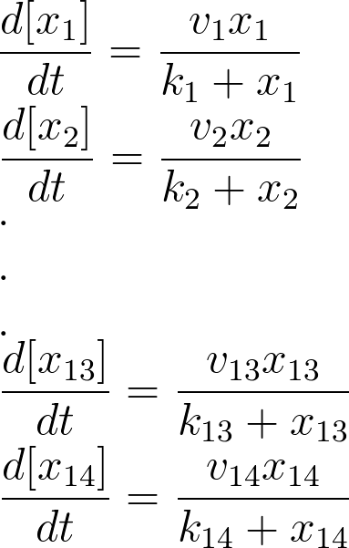
For the 14 reactions of enzyme-substrate the Michaelis-Menten kinetics is applied and we have the mass action kinetics for the three degradations. According to the kinetic laws there are 14 differential equations for enzyme-substrate reactions and three for degradations which could be constructed as:
x1 to x14 are the subtrates.
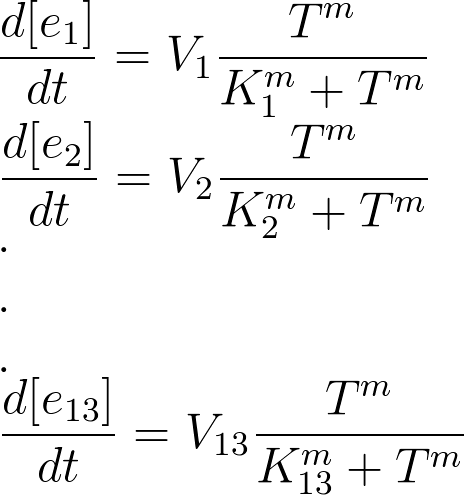
We used hill type model for enzyme temperature relations where e1 to e13 are the enzymes. Afterwards the in CellDesigner™ file was imported into Matlab. For this procedure many softwares were tested but finally the [http://www.sys-bio.org synthetic biology workbench] site used to convert the SBML model into m file. This m file was the base part for the modeling in Matlab. In this m file all the related differential equations were defined as a function with the time span and initial condition as the input. The reactions coefficients are defined by some not systemically acquired numbers to give an estimation for the reactions. These differential equations were solved by Matlab ODE function. Due to the weaknesses in CellDesigner for defining the SBML file the converted file had many problems. To solve these problems the m file was modified.
Initial solution for ODEs
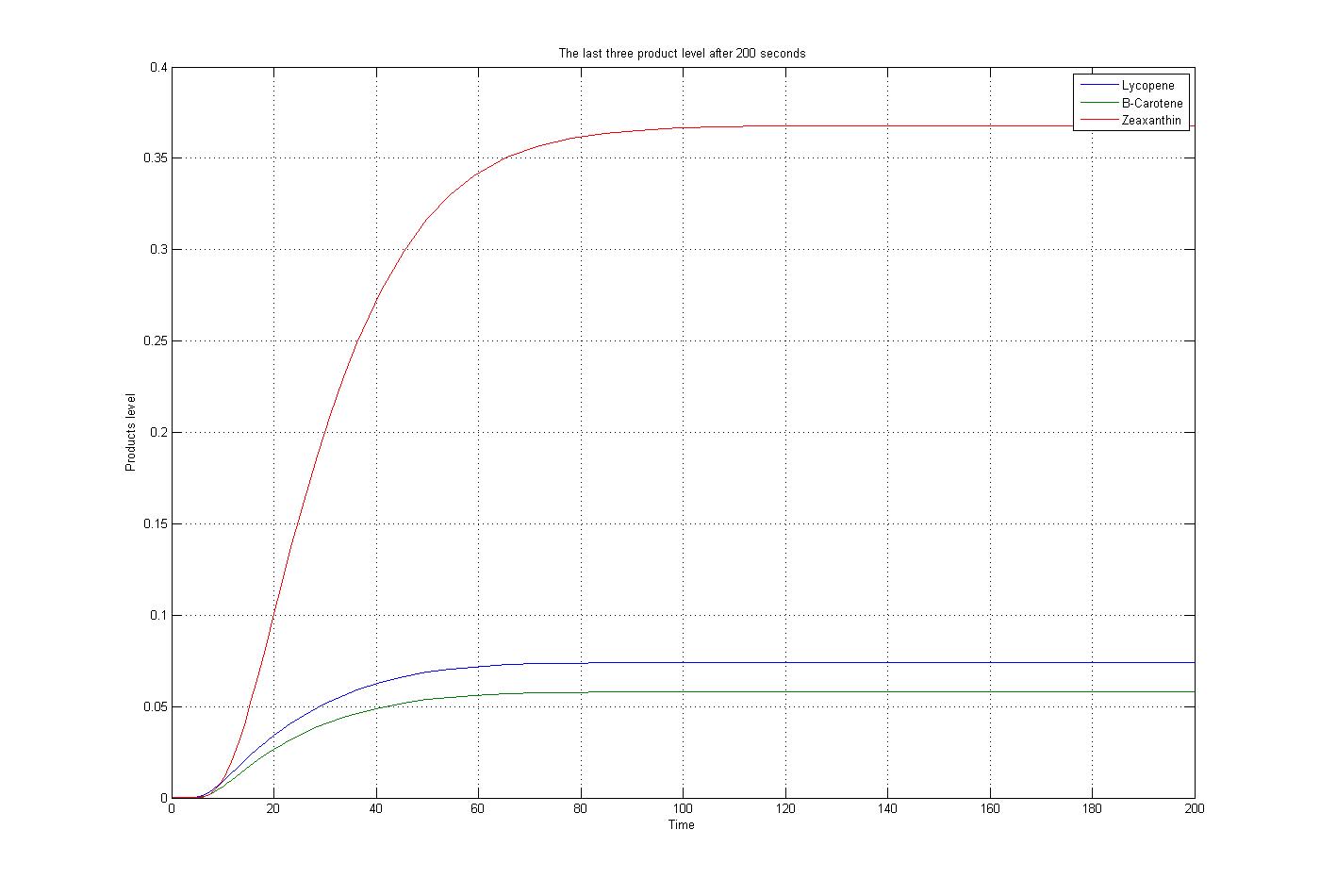
The m file function, as mentioned before, was solved by the ode15s function of Matlab. To do this procedure some assumptions were applied. The first substrate, Acetyl-CoA, assumed to produced and consumed with the same ratio. Also for simplification the level of enzymes assumed to be constant. The reaction coefficients are defined the same for all reaction with some non-accurate numbers to give an overview about the reactions. The results for these assumptions and specific boundary condition and time span of 200 seconds were plotted. These results show the steady state situation for the last three products after 200 seconds. The plot is:
Effects of the temperature on enzymes
[http://student.ccbcmd.edu/biotutorials/proteins/enzyme.html Enzymes] are catalysts that breakdown or synthesize more complex chemical compounds. They allow chemical reactions to occur fast enough to support life. Anything that an enzyme normally combines with is called a substrate. Each enzyme has an [http://student.ccbcmd.edu/biotutorials/proteins/enzyme.html optimum temperature] at which it works best. A higher temperature generally results in an increase in enzyme activity. As the temperature increases, molecular motion increases resulting in more molecular collisions. If, however, the temperature rises above a certain point, the heat will denature the enzyme, causing it to lose its three-dimensional functional shape by denaturing its hydrogen bonds. Cold temperature, on the other hand, slows down enzyme activity by decreasing molecular motion. In the monitored model the effect of temperature is important for the last three enzymes.Moreover the last three enzymes are produced on a specific temperatures to active the last three products reaction. These last three products are [http://en.wikipedia.org/wiki/Lycopene Lycopene], [http://en.wikipedia.org/wiki/Beta-carotene B-Carotene] and [http://en.wikipedia.org/wiki/Zeaxanthin Zaxanthin] which are presenting red, orange and yellow color in the environment.
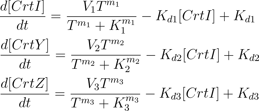
As mentioned before for the enzymes production the hill type model was used. As a result, the temperature is the main parameter in enzyme production rate. Due to degradation which is dependent on the enzyme concentration after a while the enzyme is in a stable situation.Moreover with the hill type model the enzymes work as a switch which activated on a certain temperature. The activation temperature is determined by the parameters in the hill type equation.
Lab experiments for estimating parameters
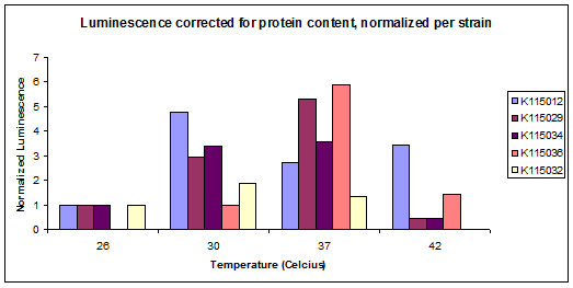
In the model, there are many parameters that were estimated arbitrary to have an initial calculation and got a feeling about the model. However to have a good model it is necessary to have a good estimation for the parameters. To find these estimation the modeling crew decided to use the results from the lab. It means that the results from lab were used to estimate parameters that not available exactly in databases. Two experiments have been designed for this procedure. The first one was an experiment for steady state situation which has been done by using Luciferase. In this experiment the enzyme activity has been measured for a specific temperature in the steady state situation.As this experiment has been done in steady state situation it was named "static". The second experiment designed to measure enzyme activity in changing situation. It means that the enzyme activities were measured in changing temperature in different time spans. As this experiment has been done in a changing situation it was named "dynamic". The results of both experiments are used to help the modeling crew to find a good estimation for parameters. An example for the lab experiment results in the steady state, which has been normalized, is shown below. These results have been used to do the calculations for the next steps.
Parameter Estimation
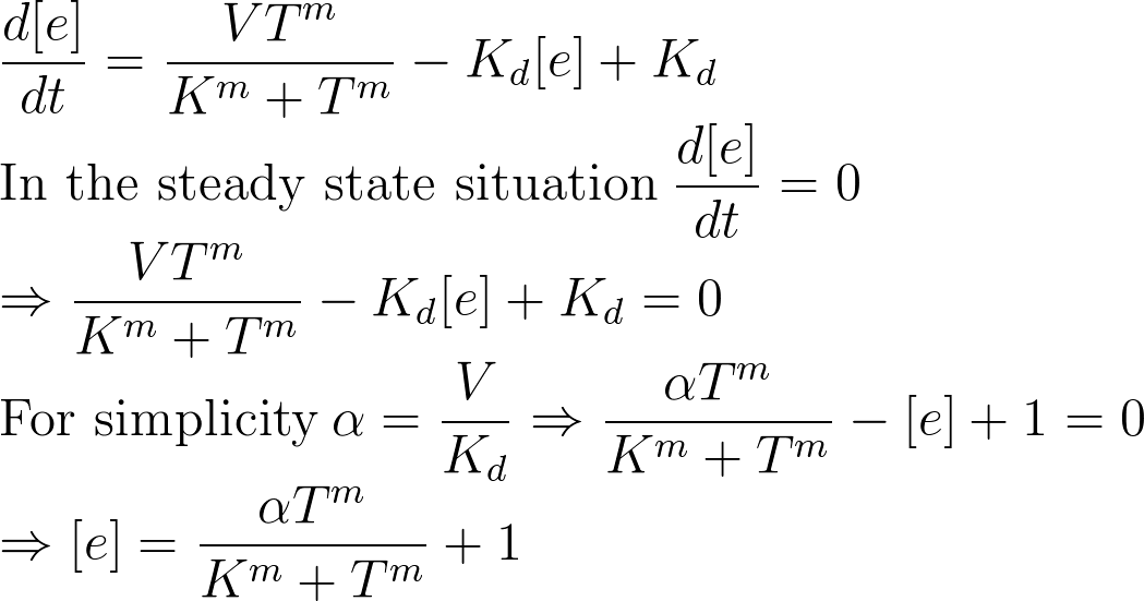
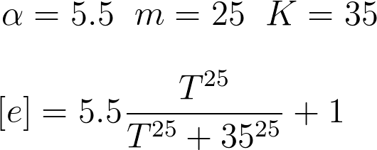
In the first step, the results from steady state situation were used to calculate the parameters. In steady state situation the enzyme concentration ratio is zero. Therefore from the lab results it is possible to derive a equation that has enzyme concentration. In this equation the enzyme concentration and temperature are known and alpha, m and K are unknown.
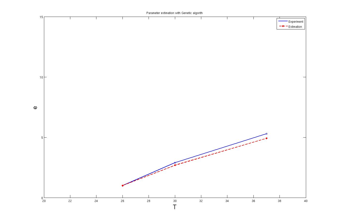
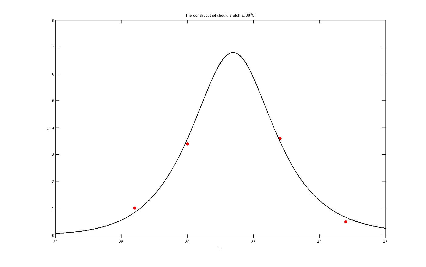
To find these parameters many solution like non linear set of equations has been tested. However the best results for the parameters has been concluded from the [http://en.wikipedia.org/wiki/Genetic_algorithm Genetic algorithm] search method. By this method parameters were estimated with a very good approximation. The calculations was based on the three points of the lab experiment results. The result for these method are shown in the below graph. The codes that used for the GA can be downloaded in Download tab.
It is clear from the graph that the result is quite good. The enzyme concentration which supposed to be active at 37°C equation is:
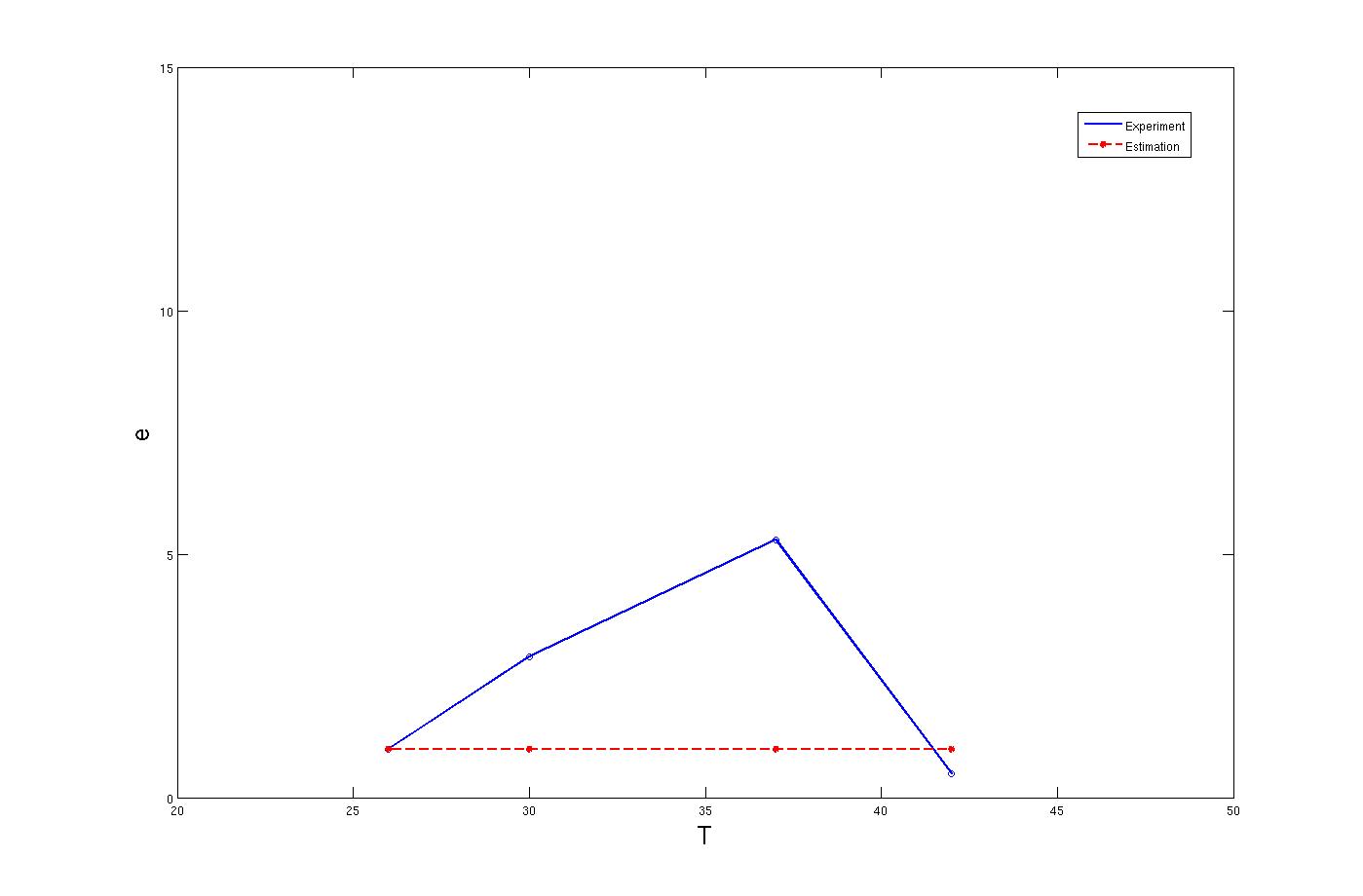
In this equation, the enzyme concentration and temperature are known but other parameters are unknown. It means that we have four points, but five unknows. In the first step we tried to solve the problem with the Genetic algorithm again. The amount of alpha consider to be known and the algorithm applied to calculate other parameters. Unfortunately results were not satisfactory.
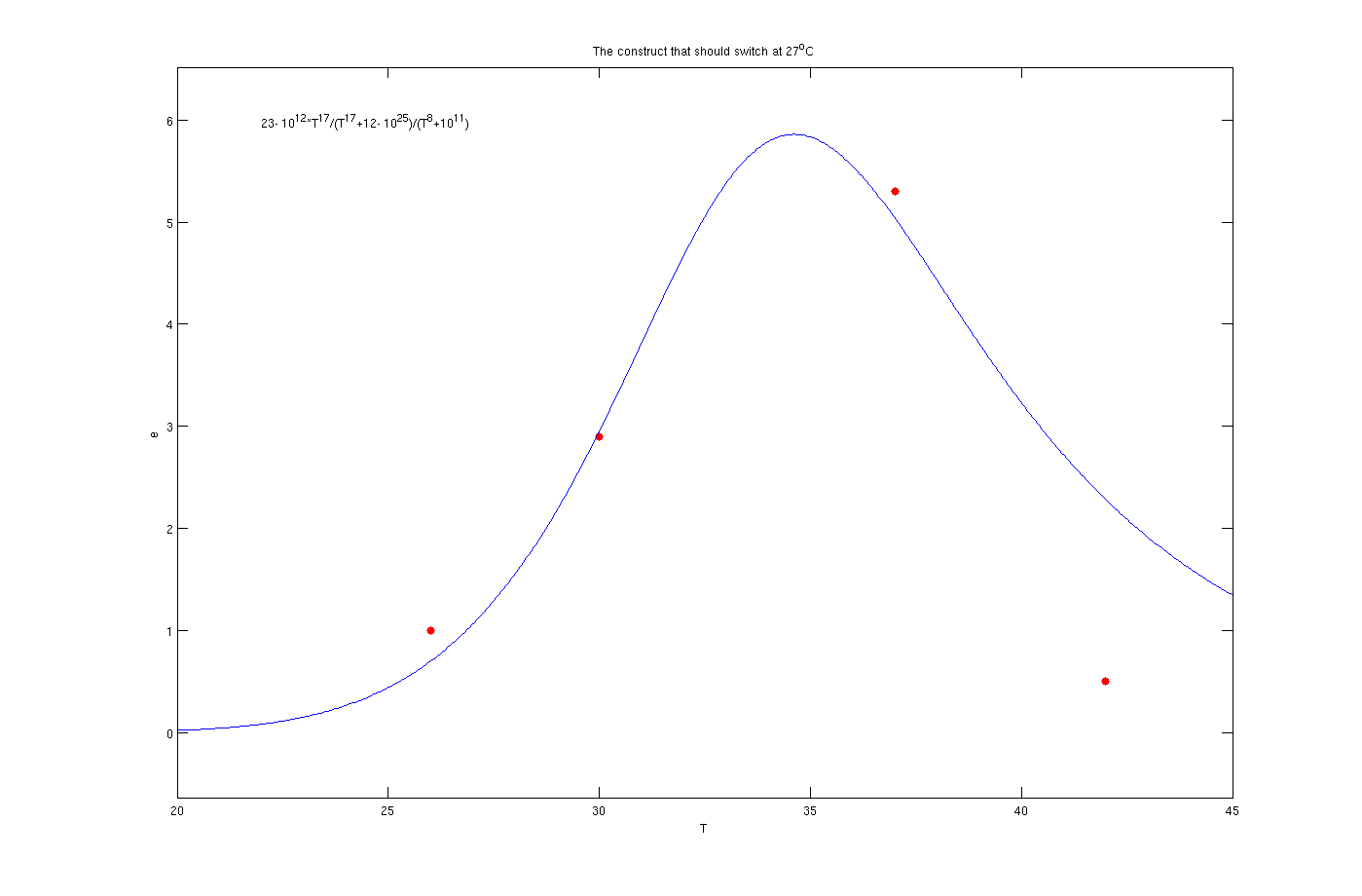
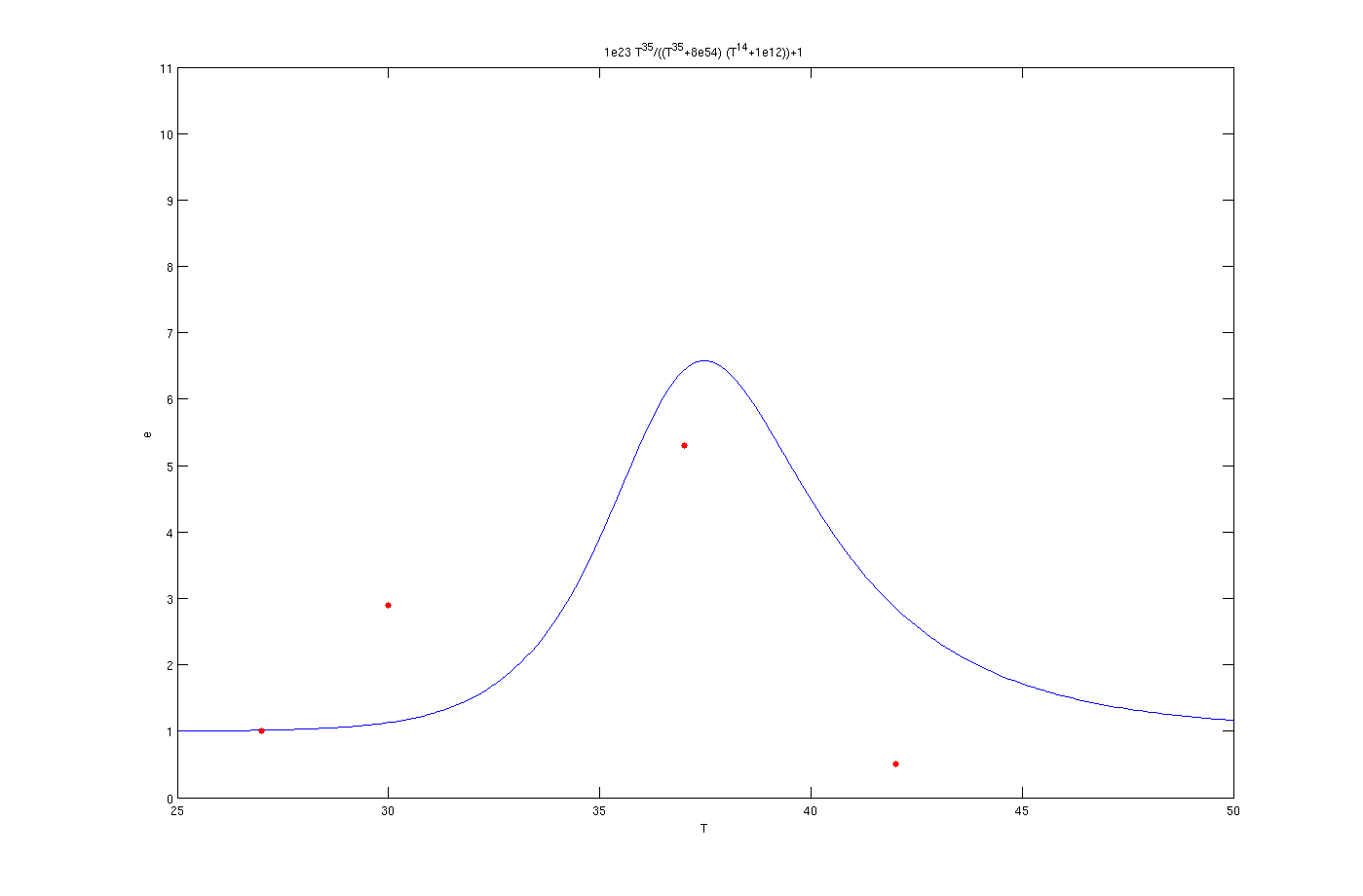
To solve this problem the try and error method has been used. Although this method is time consuming but the results are quite convincing. To use this method, one the parameters, for example m, has been assumed as known and other four was estimated by solving a set of four non linear equations. Afterwards another initially estimated parameter from the previous step assumed as known and other four has been estimated. This procedure was continued till it converged to a set of parameters. The enzyme concentrations with inhibition are:
Enzyme activates at 27°C
Enzyme activates at 30°C
Enzyme activates at 37°C
The red dots in the plots are the results from lab. It is noticeable that the models work as switches that activated in 27°C, 30°C and 37°C.
Bifurcation analysis
To have a stable system it is important to do a bifurcation analysis to find the stable ranges for different reaction parameters. This procedure has been done by defining the parameters and substrates concentration as symbolic values in Matlab. Afterwards by these symbolic values the reactions are defined in symbolic format. By these symbolic reactions a vector for reaction ratios for different substrates can be derived. Afterwards by applying a specific steady state, which has been derived from previous step but by applying the initial parameters that have been found from the databases, and changing the reactions parameters in the range that has been found from the [http://www.brenda-enzymes.info/ data base] different reaction vectors were obtained. The changes in the parameter ranges has been define by a random selection in a normal distribution between 0.001 to 0.0374. Subsequently, different vectors for reactions can be derived from this step. The [http://en.wikipedia.org/wiki/Jacobian Jacobian] applied on each vector where the derivations were respect to the substrate and product concentrations. To conclude the stability for each situation it is necessary that all the [http://en.wikipedia.org/wiki/Eigenvalue,_eigenvector_and_eigenspace eigenvalues] of each Jacobian matrix be smaller than zero. If the condition is satisfied then the reactions and pathways are in the stable situation. By this method it is possible to find an approximate ranges for the reaction parameters.
As the last three products are important and to make the life easier, a lumped model has been designed for the pathway. Two approaches has been used for this procedure. The first one was calculating all the substrates concentration on the base of the first substrate concentration. This approach makes the model too complicated therefore it has been ignored. The second approach was combining all the substrates and enzymes before Phytoene as a single reaction. It means there is a reaction that has the Acetyl-CoA as input and Phytoene. With this lumped model it is easier to calculate the stability and do the sensitivity analysis for the model.
This pathway has been modeled in Matlab and the bifurcation analysis has been done. The model has been defined in Matlab symbolic therefore by substituting the parameters, enzymes concentrations and product concentrations with numbers the stability can be derived. On the other hand the Jacobian matrix with respect to the products and substrates eigenvalues are always negative therefore it can be concluded that the pathway is always stable for the different values for parameters.
To do the sensitivity analysis on the model, the hill type equation has been implemented into the model. As a result the sensitivity of the system against the temperature has been studied in the model.
The next step is to find the coefficients of V and K for the both set of equations.
In the subtrate equations we have Vmax=Kcat . E0 where Kcat is the turnover number and E0 is the enzyme's initial concentration.
Experiment Vs Theory
... to be continued
 "
"
